Q2 - Tesla Autopilot Binary Tree Flattening Challenge
We believe a variation of this interview question has recently been asked by Tesla to full-time software engineering candidates at all levels.
As a Software Engineer at Tesla, specifically within the Autopilot division, you face the challenge of dealing with a complex stream of sensor data. This data comes in an unsorted binary tree format, capturing a wealth of information from the fleet's multitude of sensors—each critical for the immediate and strategic decisions made by the Autopilot AI.
Your task is to streamline this data flow. You are to write a function that restructures the binary tree into a flattened form
that closely resembles a singly linked list, where nodes will still have left and right pointers. More specifically, the flattened binary tree
(e.g., output singly linked list) should be in the same order as a pre-order traversal of the input binary tree. The output "singly linked list"
should use the existing BinaryTreeNode class, where the right child pointer points to the next node in the list, and the left child pointer
is set to null.
This in-place transformation is crucial: it must repurpose the existing tree structure into a linear sequence without the aid of any auxiliary data structures, such as arrays or additional lists, to hold nodes temporarily. The goal is to achieve a flattened tree with the root node as the starting point, from which the entire sequence can be traversed, reflecting the order in which the sensor data was originally structured in the tree.
The root node of the resulting flattened structure will be returned by your function, signifying the starting point of the ordered data, which now allows for streamlined and sequential access by the Autopilot system.
By accomplishing this task, you will elevate the data processing capabilities of Tesla's Autopilot, contributing to more responsive and reliable autonomous navigation.
This problem requires an in-place transformation of the binary tree, avoiding any additional auxiliary space.
Consequently, the solution aims to achieve an O(1) space complexity, which significantly adds to the difficulty of this problem!
Example 1:
Input:
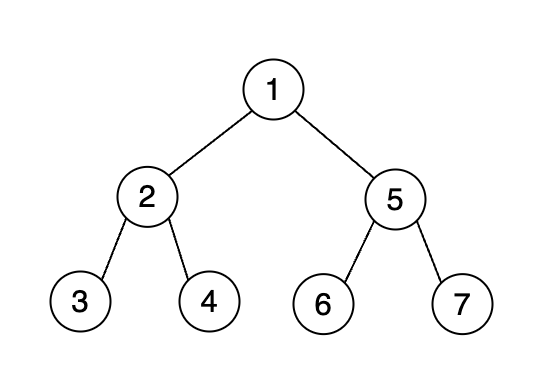
Output: Node containing the value 1
Explanation: After flattening the input binary tree, we will get:
1 --> 2 --> 3 --> 4 --> 5 --> 6 --> 7 --> [/]. Where each node's left pointer points to null, and
--> represents right pointer. The leftmost node in the flattened binary tree is the root node with value 1.
Solution 1 (For intuition only - Not Accepted in the Interview)
We will begin by exploring the most intuitive and straightforward method to tackle this problem. Let's consider the given example
of a Binary tree and observe its corresponding flattened tree in the output. What do you notice? The nodes in the flattened tree align
precisely with the pre-order traversal of the Binary Tree (or DFS traversal). If you're unfamiliar with pre-order traversal or need a refresher,
we recommend reviewing these resources for a comprehensive understanding:
resource-1 and resource-2.
Once you recognize that the flattened version of the input tree is essentially the pre-order traversal of the Binary Tree (as pointed out in the question), the most straightforward approach becomes clear. You create an additional array to hold the nodes, arranged according to their pre-order traversal. Consequently, the first element in this array will effectively represent the leftmost node in the flattened tree, which is precisely the solution sought by the question, right?
The straightforward approach involves creating an auxiliary space, such as an array, to store all the nodes in their pre-order sequence and then returning the first item in this array.
However, it's important to note that this method will not be accepted by interviewers, as it requires
additional space. The question explicitly prohibits this, instructing the interviewee to modify the given input
Binary Tree in-place instead. Moreover, we are aiming to achieve an O(1) space complexity!
Below is the solution that uses an auxiliary space as described above:
# Binary Tree Implementation.
class BinaryTreeNode:
    def __init__(self, value=0, left=None, right=None):
        self.value = value
        self.left = left
        self.right = right

# O(n) time | O(n) space
def flatten_binary_tree(root):
    if not root: return root
    pre_order_nodes = pre_order_traversal(root, [])
    # Assign the left and right pointers of each node.
    # Since it will be a 'SinglyLinkedList', left will point to None.
    for i in range(len(pre_order_nodes) - 1):
        curr_node = pre_order_nodes[i]
        next_node = pre_order_nodes[i + 1]
        curr_node.left = None
        curr_node.right = next_node

    # The leftmost node of the flattened binary tree.
    return pre_order_nodes[0]

# Helper method to populate the 'pre_order_nodes' array.
def pre_order_traversal(node, array):
    if node:
        array.append(node)
        pre_order_traversal(node.left, array)
        pre_order_traversal(node.right, array)
    return array
Complexity Analysis
- Time Complexity: O(n), where n is the number of nodes in the binary tree. Each node is visited once during the traversal, leading to a linear time complexity.
- Space Complexity: O(n), where n is the number of nodes in the binary tree. The additional array used to store the nodes in pre-order traversal results in linear space complexity.
The next solution is the accepted approach that ingeniously transforms the array in-place, eliminating the need for any auxiliary space. This is the real challenge that elevates the difficulty level of this question. It encompasses numerous intricate aspects that require careful consideration to devise the solution presented below. We highly recommend using pen and paper to thoroughly understand and internalize the underlying logic.
Solution 2 (Expected Solution)
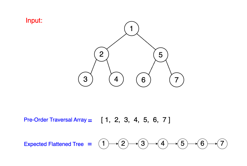
Take a look at the example below. For the input Binary Tree shown, we can see the pre-order traversal array and a flattened tree with the
leftmost node valued at 1, which is our target output. It's important to observe that the node order in the flattened tree output precisely matches the
pre-order traversal array as we've already discovered in our first solution. The subtle yet significant difference is that in the flattened tree,
each node's left and right pointers have been updated to mirror the linear sequence of the array. But how do we transform the input binary tree into a
flattened tree without depending on the pre-order traversal array? This is the challenge that we need to address.
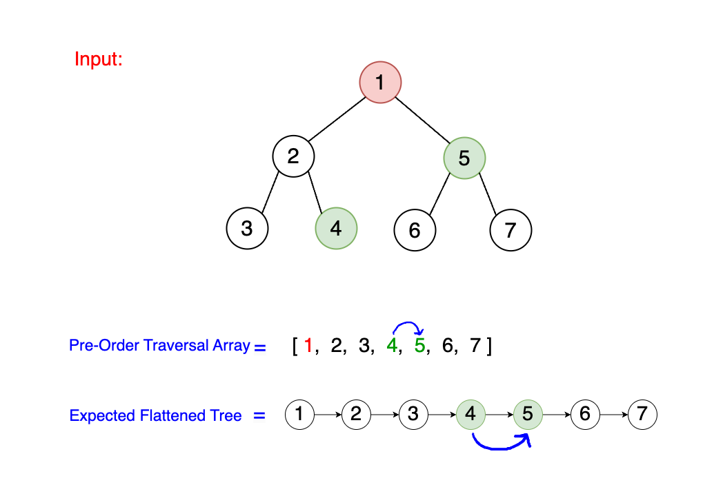
Let's zoom in on the left and right neighbors—or children—of a node in our flattened tree, for instance,
the node with value 1. After flattening, its right child is the node with value 2, and its left child is null.
Take a moment here. What do you notice? Take a look at the diagram below. Where are the nodes 4 and 5 located with respect to the node
1 in the original binary tree?
In our original binary tree:
4is the rightmost child of1's original left subtree. You will see why that matters soon!5is the right child of1. Hence, node5is now node4's right child in the flattened tree.
In pre-order traversal, or DFS traversal, whenever we consider a root node, by definition of DFS, the very last node discovered on the root node's left sub-tree (the rightmost node of the left subtree) will precede the immediate right child of the root node. This is because in DFS, we fully explore the left subtree before moving to the right child of the root node.
We will now walk through this solution step-by-step with detailed explanations and visual demonstrations at each stage. We'll use the provided example tree above.
1) Initialization and First Iteration
- We start with the root node (
1). - Check if
root.leftis notNone(it is2in this case). - Then, we call the helper method
get_rightmost_node(root.left)to find therightmostnode of the left subtree of node 1 (remember that this will be the last visited node in the left subtree before moving to the right subtree). - We find that
4is the rightmost child of1's original left subtree.
Below is the code snippet demonstrating the process of finding the rightmost node of a given node's left subtree:
Finding the Rightmost Node of a Given Node's Left Subtree
# Main function.
def flatten_binary_tree(root):
    while root:
        # If the current node has a left child, find the rightmost node of this left subtree.
        if root.left:
            # For the tree:
            #     1
            #    / \
            #   2   5
            #  / \ / \
            # 3  4 6  7
            # Node 4 is the rightmost node in the left subtree of node 1.
            # Find the rightmost node of the left subtree using the helper method.
            left_subtree_right_most = get_rightmost_node(root.left)
            ...

# Helper method to find the rightmost node of a given subtree.
def get_rightmost_node(node):
    if not node:
        return node
    # Traverse to the extreme right of the subtree.
    while node.right:
        node = node.right
    return node
What do we know about this node 4? In pre-order traversal, this node will appear right before the root node's (1) original right child, which is node 5.
Thus, node 4 needs to be connected to node 5 in the flattened tree. You can see this in the below diagram. Node 5 will become the right child of
node 4 at the end of the first iteration:
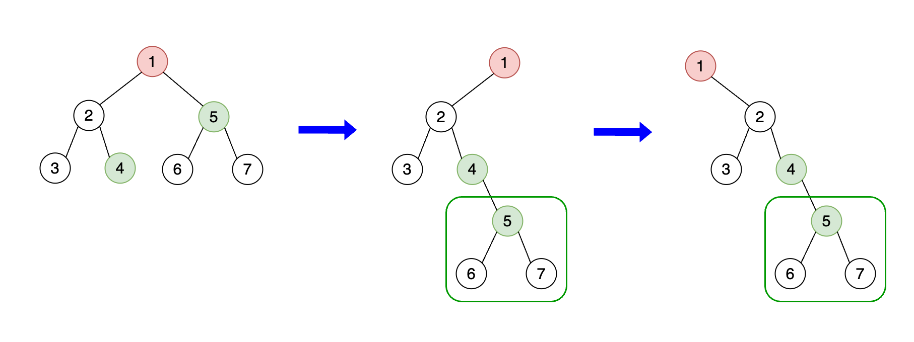
At any given iteration, when we consider the current node, the rightmost node of the current node's left subtree will always be connected to the
current node's immediate right child. For instance, in our example with the root node 1, the rightmost node of its left subtree is 4. During the iteration,
node 4 will be connected to node 1's immediate right child, which is 5. This ensures that the flattened tree maintains the correct pre-order traversal sequence.
The diagram above demonstrates this!
Moreover, notice that we convert the updated left subtree of the root node 1 into its new right subtree, while setting its left child to null, in accordance
with the question's requirements. Below is the code snippet responsible for this transformation:
Moving the Updated Left Subtree of the Current Node into its New Right Subtree
# Main function.
def flatten_binary_tree(root):
    while root:
        # If the current node has a left child, find the rightmost node of this left subtree.
        if root.left:
            # For the tree:
            #     1
            #    / \
            #   2   5
            #  / \ / \
            # 3  4 6  7
            # Node 4 is the rightmost node in the left subtree of node 1.
            # Find the rightmost node of the left subtree using the helper method.
            left_subtree_right_most = get_rightmost_node(root.left)

            # The rightmost node's right child should point to the current node's right child.
            left_subtree_right_most.right = root.right

            # Move the entire left subtree (updated above) to the right.
            root.right = root.left

            # After the above updates, the tree will look like this:
            #     1
            #      \
            #       2
            #      / \
            #     3   4
            #          \
            #           5
            #          / \
            #         6   7
            # Set the left child of the current node to 'None' as we are making it a singly linked list.
            root.left = None

        # Move to the right child of the current node and repeat the process.
        root = root.right
With the completion of the first iteration, we have successfully restructured the initial portion of our binary tree. The next step involves moving to the new right child
of the current root node (1), which is node 2, and repeating this process. This ensures that each subtree is flattened in a similar manner, ultimately achieving the
desired pre-order traversal sequence for the entire tree. Let's now move on to the second iteration and observe how the tree continues to transform.
2) Second Iteration
Moving to the next iteration, our new root node is now 2. Let's follow the same steps we discussed previously to flatten this subtree.
- Current node (
2). - Check if
root.leftis notNone(it is3in this case). - Call the helper method
get_rightmost_node(root.left)to find therightmostnode of the left subtree of node 2. - We find that
3is the rightmost child of2's left subtree.
Now, let's visualize this:
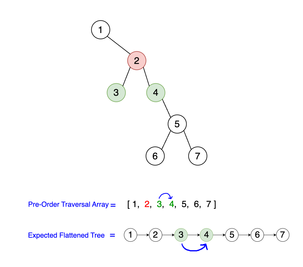
What do we know about this node 3? Again, in pre-order traversal, it will appear right before our current root node's (2) right child, which is node 4.
Thus, node 3 needs to be connected to node 4 in the flattened tree. You can see this in the below diagram. Node 4 will become the right child of
node 3:
Once again, when we consider the current node, the rightmost node of the current node's left subtree will always be connected to the
current node's immediate right child. For instance, in our example with node 2, the rightmost node of its left subtree is 3. During the iteration,
node 3 will be connected to node 2's immediate right child, which is 4. This ensures that the flattened tree maintains the correct pre-order traversal sequence.
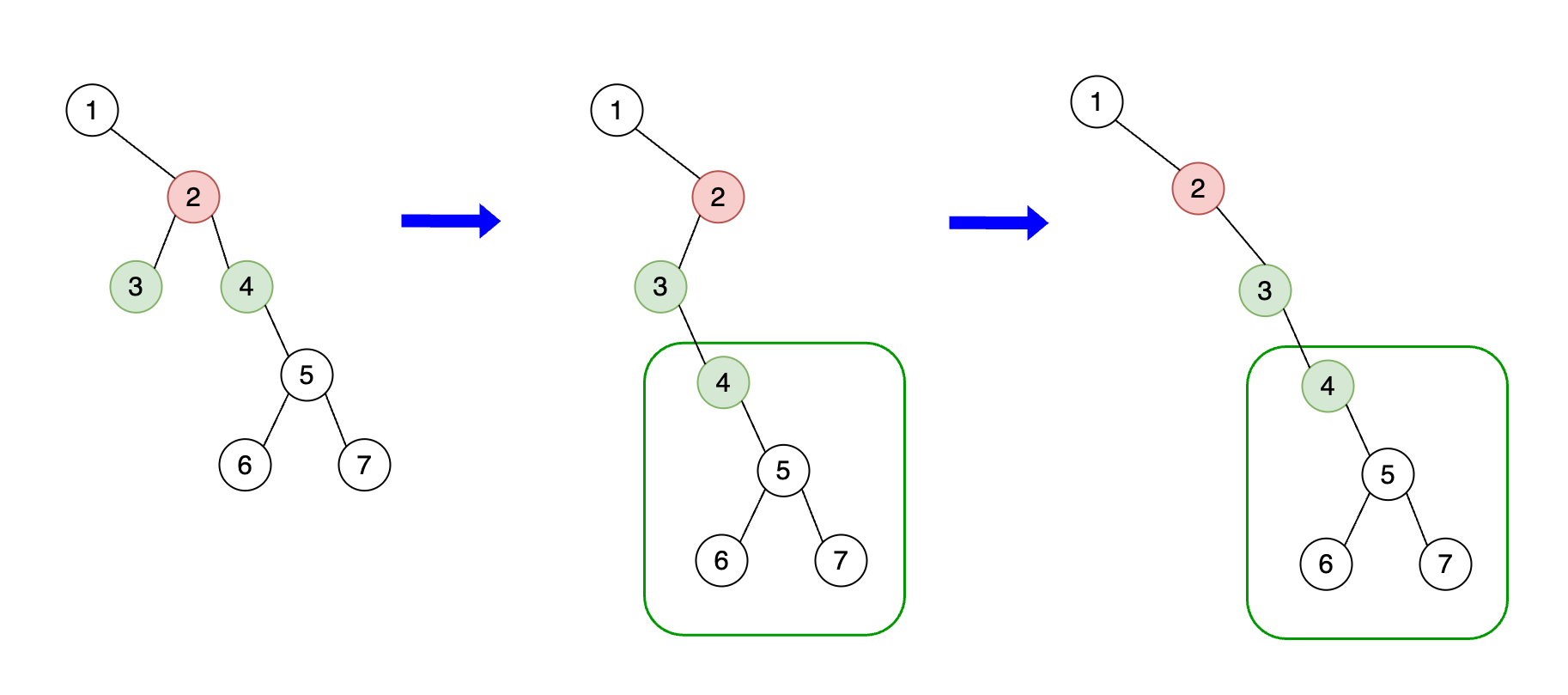
Moreover, notice that we convert the updated left subtree of node 2 into its new right subtree, while setting its left child to null, in accordance
with the question's requirements.
After the second iteration, the tree continues to transform, ensuring the pre-order sequence is maintained. The tree now looks like this:
By repeating this process, the entire binary tree will eventually be flattened into a singly linked list that follows the pre-order traversal sequence. Each subtree is processed in a similar manner, ensuring that every node's left child is set to null and its right child points to the next node in the pre-order traversal.
With this understanding, let's proceed to the third iteration and continue transforming the binary tree into a flattened singly linked list.
3) Third and Fourth Iterations
In these iterations, we process nodes 3 and 4. Let's examine each step in detail:
Third Iteration:
- Current node (
3). - Check if
root.leftis notNone.
For node 3, there is no left child, so the condition if root.left: is not satisfied. There is no need for any modification here because node 3 is already correctly positioned in the flattened tree. We move on to the next node in the sequence, which is node 4.
Fourth Iteration:
- Current node (
4). - Check if
root.leftis notNone.
Similarly, node 4 does not have a left child, so the condition if root.left: is not satisfied. Again, there is no need for any modification because node 4 is already in the correct
place in the pre-order sequence.
In both of these iterations, the nodes are already correctly positioned in the flattened tree, so no further actions are necessary. This can be visualized in the following diagram:
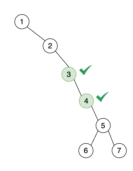
As shown, nodes 3 and 4 are already in their correct places in the pre-order sequence. Therefore, we move to the right child of node 4, which is node 5.
With these iterations complete, we can now proceed to the next steps of the algorithm, continuing to transform the binary tree into a flattened singly linked list.
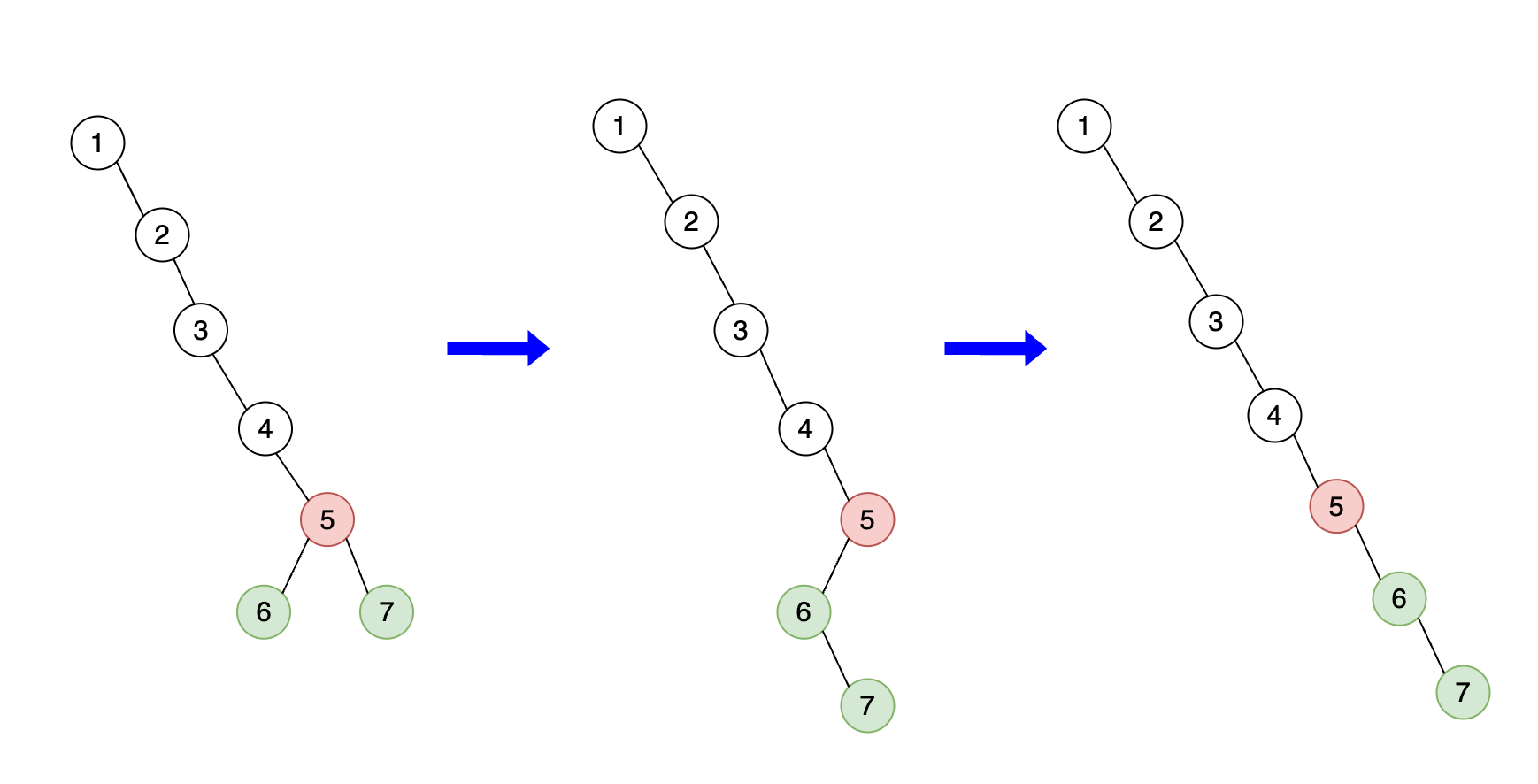
4) Fifth Iteration
Moving to the next iteration, our new root node is now 5. Let's follow the same steps we discussed previously to flatten this subtree.
- Current node (
5). - Check if
root.leftis notNone(it is6in this case). - Call the helper method
get_rightmost_node(root.left)to find therightmostnode of the left subtree of node 5. - We find that
6is the rightmost child of5's left subtree.
Now, let's visualize this:
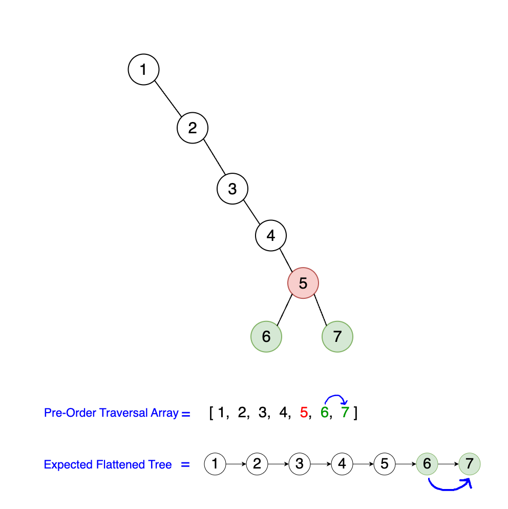
What do we know about this node 6? Again, in pre-order traversal, it will appear right before our current root node's (5) right child, which is node 7.
Thus, node 6 needs to be connected to node 7 in the flattened tree. You can see this in the below diagram. Node 7 will become the right child of
node 6:
Once again, when we consider the current node, the rightmost node of the current node's left subtree will always be connected to the
current node's immediate right child. For instance, in our example with node 5, the rightmost node of its left subtree is 6. During the iteration,
node 6 will be connected to node 5's immediate right child, which is 7. This ensures that the flattened tree maintains the correct pre-order traversal sequence.
Once again, we convert the updated left subtree of node 5 into its new right subtree, while setting its left child to null, in accordance
with the question's requirements. The tree now looks like this:
5) Sixth and Seventh Iterations
In these iterations, we process nodes 6 and 7. Let's examine each step in detail:
Sixth Iteration:
- Current node (
6). - Check if
root.leftis notNone.
For node 6, there is no left child, so the condition if root.left: is not met. Since node 6 is already correctly positioned in the flattened tree, no modifications are needed.
We then move to the next node in the sequence, which is node 7.
Seventh Iteration:
- Current node (
7). - Check if
root.leftis notNone.
Similarly, node 7 does not have a left child, so the condition if root.left: is not satisfied. Again, there is no need for any modification because node 7 is already in the correct
place in the pre-order sequence.
During these iterations, nodes 6 and 7 are already positioned correctly in the flattened tree, so no further actions are required. This is illustrated in the following diagram:
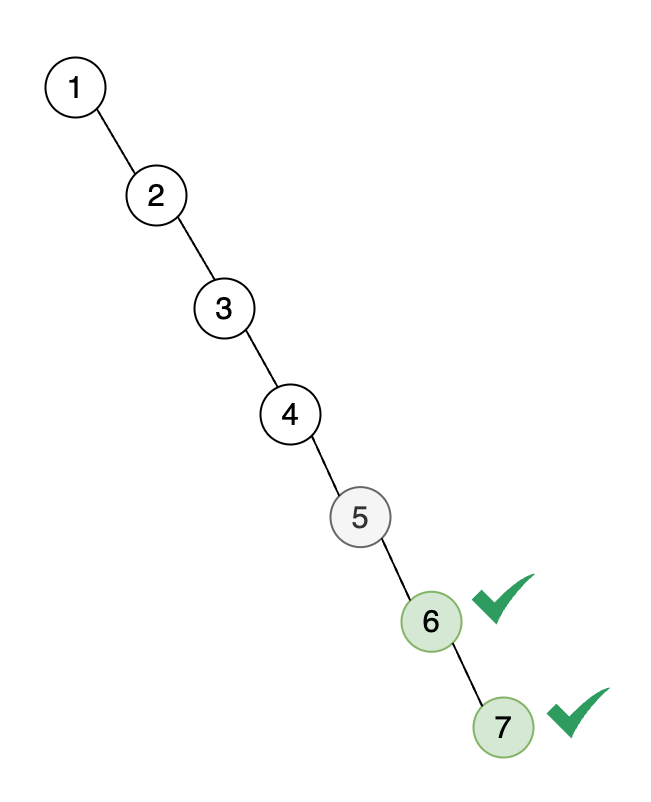
As shown, nodes 6 and 7 are already in their correct places in the pre-order sequence. Therefore, we move to the right child of node 7, but since there are no more nodes
left, our algorithm ends here. With these iterations complete, the entire binary tree has been successfully transformed into a flattened singly linked list following the
pre-order traversal sequence.
Complexity Analysis:
-
Time Complexity: O(n), where N represents the number of nodes in our binary tree.
Explanation:
-
Traversing Nodes
- The algorithm processes each node exactly once. During each iteration, it performs a constant amount of work (checking for a left child, finding the rightmost node in the left subtree, reassigning pointers). Thus, the time complexity is O(n).
-
Finding Rightmost Nodes
- Although finding the rightmost node in the left subtree involves a loop, it doesn't change the overall time complexity. Each node is visited at most twice (once during the main while loop and once during the traversal to find the rightmost node), so the complexity remains O(n).
-
Traversing Nodes
-
Space Complexity: O(1)
Explanation:
-
In-Place Transformation
- The algorithm modifies the tree in place without using any extra space proportional to the number of nodes. It uses a constant amount of extra space for variables
such as
left_subtree_right_mostand the pointers being reassigned. Hence, the space complexity is O(1).
- The algorithm modifies the tree in place without using any extra space proportional to the number of nodes. It uses a constant amount of extra space for variables
such as
Finding an O(1) space solution is particularly challenging because it requires in-place modification of the tree structure. This level of space efficiency often involves intricate manipulation of pointers and traversal methods. Morris Traversal is a renowned algorithm that achieves such space efficiency. For those curious to learn more about Morris Traversal and its space-efficient approach to tree traversal, you can read further here.
-
In-Place Transformation
Below is the coding solution for the algorithm we've just explored. With the insights and understanding gained, this should now be much clearer to the readers:
# Binary Tree Implementation.
class BinaryTreeNode:
    def __init__(self, value=0, left=None, right=None):
        self.value = value
        self.left = left
        self.right = right

# O(n) time | O(1) space
def flatten_binary_tree(root):
    while root:
        # If the current node has a left child, find the rightmost node of this left subtree.
        if root.left:
            # For the tree:
            #     1
            #    / \
            #   2   5
            #  / \ / \
            # 3  4 6  7
            # Node 4 is the rightmost node in the left subtree of node 1.
            # Find the rightmost node of the left subtree using the helper method.
            left_subtree_right_most = get_rightmost_node(root.left)

            # The rightmost node's right child should point to the current node's right child.
            left_subtree_right_most.right = root.right

            # Move the entire left subtree (updated above) to the right.
            root.right = root.left

            # After the above updates, the tree will look like this:
            #     1
            #      \
            #       2
            #      / \
            #     3   4
            #          \
            #           5
            #          / \
            #         6   7
            # Set the left child of the current node to 'None' as we are making it a singly linked list.
            root.left = None

        # Move to the right child of the current node and repeat the process.
        root = root.right

# Helper method to find the rightmost node of a given subtree.
def get_rightmost_node(node):
    if not node:
        return node
    # Traverse to the extreme right of the subtree.
    while node.right:
        node = node.right
    return node
Final Notes
We believe this question has been asked frequently by Tesla in recent interviews! It exemplifies the sort of complex data structuring and in-place algorithmic transformations that are critical for handling high-volume, real-time data streams in autonomous vehicle systems.
Aspiring to join Tesla's Autopilot team as a software engineer requires not only a strong grasp of data structures and algorithms but also the ability to apply these concepts to enhance system performance and reliability. This challenge of transforming a binary tree into a flattened singly linked list encapsulates several important lessons and strategies:
-
Understanding Autopilot Data Flow: The task underscores the necessity for efficient data processing mechanisms in Tesla's Autopilot system. A well-structured data flow is crucial for the rapid decision-making processes required in autonomous driving.
-
In-Place Transformations: The constraint of modifying the binary tree in-place, without auxiliary data structures, mirrors the memory and processing efficiency goals in embedded systems such as those in Tesla's vehicles.
-
Algorithmic Ingenuity: Tesla values innovative problem-solving approaches. This challenge encourages thinking beyond conventional methods, showcasing how recursive in-place transformations can lead to optimal solutions.
-
Space Complexity Considerations: By focusing on in-place operations, the challenge aligns with the real-world scenario of hardware limitations in Tesla's on-board systems, where optimizing space complexity is as critical as time complexity.
-
Practical Application of Theoretical Concepts: The problem serves as a bridge between theoretical data structure manipulation and practical application in systems like Tesla's Autopilot, where such transformations may optimize sensor data utilization.
-
Adaptability in Algorithm Design: The question assesses the candidate's adaptability in algorithm design, reflecting Tesla's dynamic approach to engineering challenges in the ever-evolving field of autonomous driving.
-
Effective Communication of Solution Strategy: Articulating a complex algorithm clearly is essential. This skill is indicative of the ability to work collaboratively in Tesla's interdisciplinary teams, where clear communication drives innovation.
-
Specificity to Tesla's Needs: Tailoring your solution to the context of Tesla's Autopilot system can demonstrate an understanding of how such algorithmic problems are not mere academic exercises but are directly applicable to the company's technological challenges.
In preparing for a software engineering role at Tesla, especially within the Autopilot division, it is imperative to display a combination of technical prowess and the innovative application of these skills. Challenges like the binary tree flattening are reflective of real-world problems that could directly impact the efficiency and effectiveness of Tesla's Autopilot system. Your ability to navigate such challenges with efficient, in-place algorithms can set you apart as a candidate who is not only technically proficient but also cognizant of the practical implications of their work in the context of Tesla's mission.
Keep innovating and drive forward the future of autonomous transportation!
Good luck with your interview preparation!