Q1 - Google Server Traffic Management
We believe a variation of this interview question has recently been asked by Google to full-time software engineering candidates for different positions.
In the complex server networks of Google, managing the flow of information is critical to ensure high availability and efficient data processing. Your team is tasked with developing an algorithm to manage data packet distribution across server racks represented in a two-dimensional grid.
Each server rack within the grid can either transmit a data packet, allowing it to continue upward, or force it to split and find alternate routes if it's occupied. Each cell in the grid can either be a switch (S), an empty space (E), an amplifier left (FL), or an amplifier right (FR).
- An E represents an empty space that allows a data packet to pass through vertically.
- An S represents a switch that behaves like a block, forcing the data packet to split and find alternate routes if possible. If no path is available, the packet is lost.
- An FL represents an amplifier that multiplies the data packet by a specified factor and directs it to the left. If the left path is blocked, it moves forward.
- An FR represents an amplifier that multiplies the data packet by a specified factor and directs it to the right. If the right path is blocked, it moves forward.
- If a data packet encounters an FL or FR on its way in the same row (not directly above), it acts as an E by allowing the packet to pass through, but also amplifies the packet. The direction remains whatever it was before.
- There can be at most one FL or FR in each row and column.
The data packets start at a specific point in the bottom row with a given amount of data (in TB). If a data packet encounters an empty space (E), it continues upward. If it hits a switch (S), it behaves like a block, forcing the data to split to the left and right. If it encounters an amplifier (FL) or (FR), the data packet is multiplied by the amplifier's factor and continues in the respective direction. If there are blocks in both directions, it proceeds upward like an (E).
The grid's bottom row is guaranteed to be empty spaces (E). The top row can contain a mix of empty spaces (E) and switches (S).
Write a function that simulates the behavior of the data packets as they traverse the grid and returns the total amount of data (in TB) that exits from the network grid at the top together with their distribution among the cells in the top row as a list.
We believe this question is among the most challenging ones recently asked by Google. Please be aware that Google recognizes the difficulty of this problem. We believe interviewees are given approximately 60 minutes to solve it.
Example 1
Input:
server_grid = [
    ['E', 'E', 'E', 'S', 'E'],
    ['E', 'FL', 'S', 'S', 'E'],
    ['E', 'E', 'FR', 'S', 'E'],
    ['S', 'S', 'E', 'E', 'S'],
    ['E', 'E', 'E', 'E', 'E'],
],
entry_point = 1,
data_amount = 500  # in TB,
amplifier_factor = 2

Output:
[500, [500, 0, 0, 0, 0]]
Example 1 Visualization
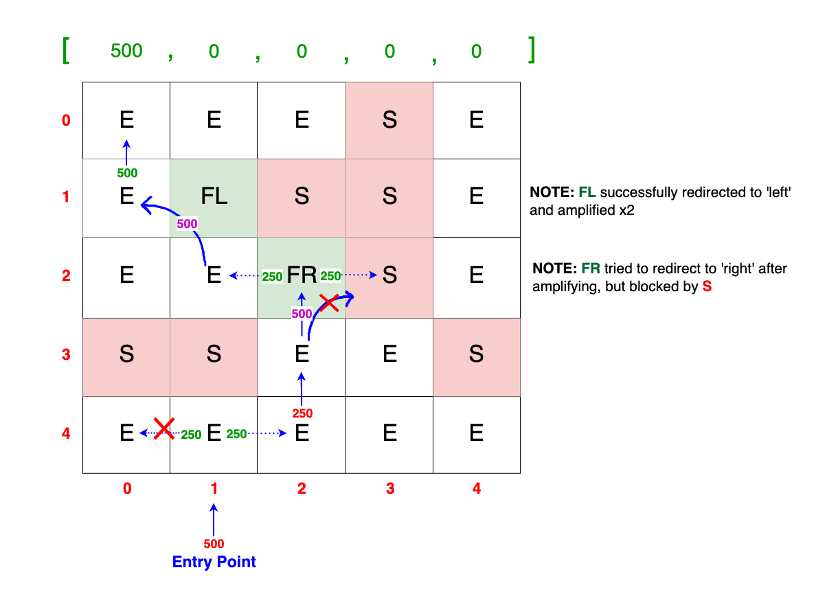
Pay close attention to the scenario where the packet, initially at 500 TB at (row=4, col=1), encounters a block at (row=3, col=1). As expected, the packet's value is halved to 250 TB. However, an important detail to note here is that only the right packet flow continues; the left flow is effectively blocked at (row=4, col=0) and lost.
Example 2
Input:
server_grid = [
  ['E', 'E', 'E', 'E', 'S'],
  ['S', 'E', 'S', 'E', 'FL'],
  ['E', 'E', 'E', 'E', 'E'],
  ['E', 'S', 'E', 'E', 'E'],
  ['E', 'E', 'E', 'E', 'E'],
]
entry_point = 1,
data_amount = 1000  # in TB,
amplifier_factor = 1.5

Output:
[750.0, [0, 500.0, 0, 250.0, 0]]
Example 2 Visualization
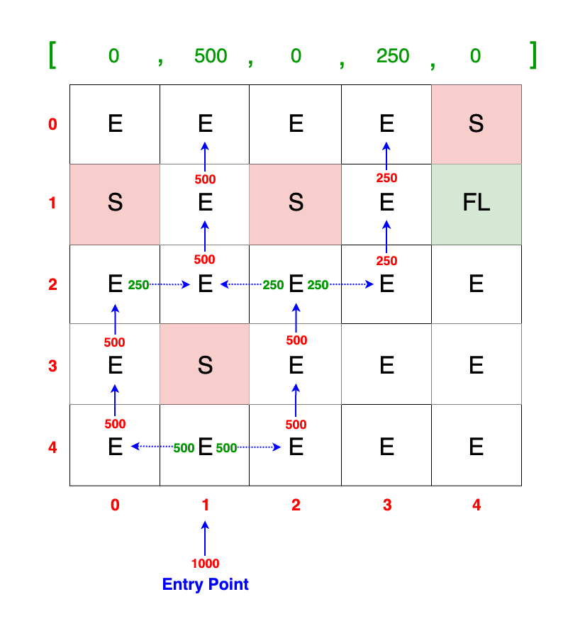
Notice that the packets at (row=2, col=0) and (row=2, col=2) are both 250 TB. These accumulate at
(row=2, col=1) to form a combined total of 500 TB.
This accumulation illustrates how the packets converge and sum up when they encounter a common cell without a block.
Solution
In this problem, we're tasked with simulating the flow of network packets through a grid. The core of our algorithm lies in handling this flow realistically, adhering to the rules of physics and the nuances of real-world packet distribution. The fundamental principle of our approach is a two-row iterative process: at each step, we only consider two rows—the current row for updating packet percentages and the previous row (e.g., row below the current one) to inform these updates.
This method captures the dynamic nature of packet flow, allowing us to track how packets, starting at a specific value from the source in TB, navigate through the grid, split when encountering switches, and possibly merge in subsequent cells. The challenge and intricacy of this solution arise from the various edge cases inherent in this kind of simulation. Each cell in the grid can either allow a packet to pass through (E), block it, or cause it to split and change directions (S) or amplify it and change its direction or amplify it without any direction change (FL/FR). How the packets split and flow depends heavily on the immediate layout of the grid around them, making each step a complex decision point.
With this overview in mind, we can proceed to explore each aspect of the algorithm in more detail, starting from the initial packet distribution, moving through the rules governing packet flow and splits, and culminating in the handling of various edge cases.
What makes this question particularly challenging is the number of edge cases that we need to consider. Google is aware of this, and it's okay to ask for guidance on this problem. That's why you are given ~60 minutes.
1) Initialization of the Starting Row
Since the network data packets start from the last row and move upwards, the initial row is actually the last row (i.e., where the entry point is).
# Main function.
def data_packet_distribution(server_grid, entry_point, data_amount, amplifier_factor):
    rows = len(server_grid)
    cols = len(server_grid[0])

    # Last row will have a cell (entry) from which
    # data packet will move up. Hence, we update the cell value to 'data_amount'.
    below_data_row = [0] * cols
    below_data_row[entry_point] = data_amount
    ...
As per the question prompt, the last row - the starting row - will always be composed of 'E's, indicating that the packet can flow from any of the cells in the starting row.
However, there will only be one entry point, as given by the entry_point parameter. As you can see from the code snippet above, we create a new array - below_data_row - that corresponds to
the starting row. Since our initial matrix contains strings, we need to create an additional array of the same length as the columns, which will contain 0s everywhere except at the entry_point.
We update the array value at the entry_point to the given data_amount, effectively marking that we have all of the packets coming in at the beginning.
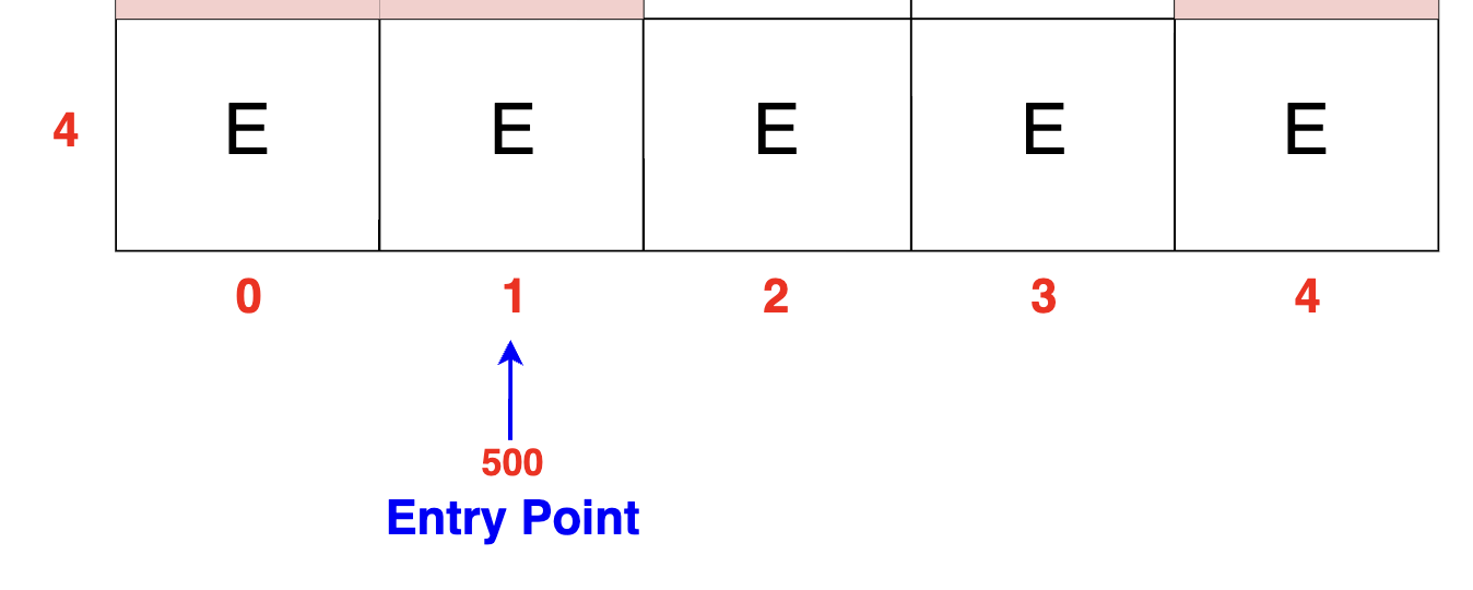
The diagram below shows the initial row in Example-1. We are updating the entry cell to contain the total amount of packets:
2) The Two-Row Approach
The core of our algorithm is the two-row approach, where at each step, we only need to consider two rows:
- The Previous Row (
below_data_row): This row holds the packet distribution from the previous iteration, which informs the updates to the current row. - The Current Row (
curr_data_row): This is the row we're currently updating with new packet amount based on the row below.
At each step, the algorithm calculates the distribution of packets in the current row based on the distribution in the row below it. This approach ensures that we're only ever working with a manageable subset of the entire grid, leading to efficient computation and easier handling of the various packet flow scenarios.
The following code snippet demonstrates this approach:
# Main function.
def data_packet_distribution(server_grid, entry_point, data_amount, amplifier_factor):
    rows = len(server_grid)
    cols = len(server_grid[0])

    # Last row will have a cell (entry) from which
    # data packet will move up. Hence, we update the cell value to 'data_amount'.
    below_data_row = [0] * cols
    below_data_row[entry_point] = data_amount

    for r in range(rows - 2, -1, -1):
        # At each iteration, 'curr_data_row' is what we are trying to update
        # using values from 'below_data_row'.
        curr_data_row = [0] * cols
        for c in range(cols):
            # ... processing for packet distribution

        below_data_row = curr_data_row
Here, for each row r in the grid (array), we assign curr_data_row to be the current row we're working on. Again, we are initializing it with 0s as usual.
We use below_data_row, which holds the packet distribution from the previous iteration, to determine how packets in curr_data_row should be distributed. After processing the current row,
we set below_data_row to be curr_data_row, effectively moving one row up the grid for the next iteration. This method mirrors the realistic propagation of packets through a network, where
the behavior at each node depends directly on the immediate inputs it receives, rather than the entire network's state, etc.
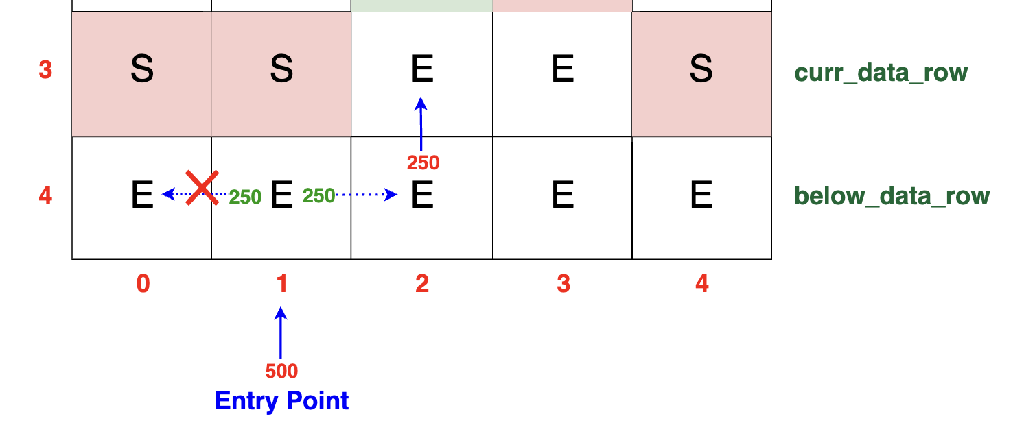
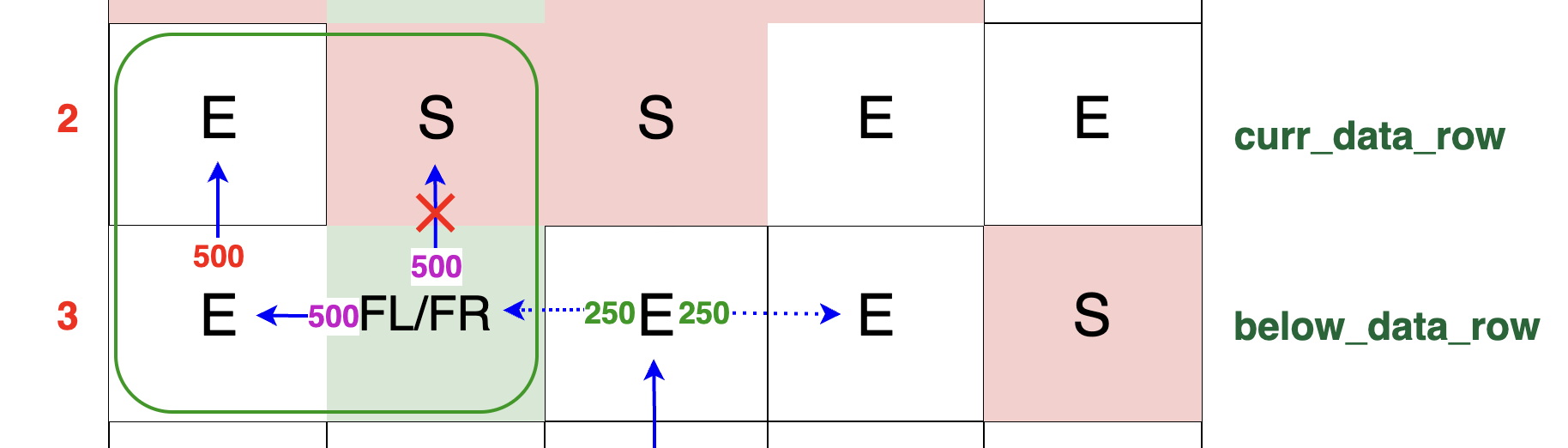
The diagram below illustrates how the data distribution in a cell of the current row is directly influenced by the row below it. In this specific example,
the current cell holds a value of S, signifying that packets located directly below need to split due to the presence of a switch. Consequently, half of the packets
move to the left and the other half move to the right. The packets moving to the left are completely lost due to another switch; the packets moving to the right can move
directly upward since the cell in the current row is free (E). Hence, only half of the total packet amount (e.g., 250 TB) reaches our curr_data_row.
We iterate through each row up to the first one, where the packets exit the grid. The remaining amount of data in these final row cells represent our solution, indicating how packets are distributed across the grid.
In the upcoming sections, we'll delve into each specific case that the algorithm must consider to accurately simulate packet flow and distribution.
3) No Packet Flow from Above
We iterate through each cell c in the current row (curr_data_row). For each cell, we first check the status of the cell directly below it in the previous row (below_data_row[c]).
This check is performed to ascertain whether there is any packet at c in below_data_row that can flow up to curr_data_row[c].
Here's the relevant code snippet:
for r in range(rows - 2, -1, -1):
    # At each iteration, 'curr_data_row' is what we are trying to update
    # using values from 'below_data_row'.
    curr_data_row = [0] * cols
    for c in range(cols):
        # There is no packet below to go up.
        if below_data_row[c] == 0:
            continue
    ...
What does below_data_row[c] == 0 indicate?
1) The Cell Below is a Switch (S): If the below cell in the original grid is S, it signifies the presence of a switch. In this scenario, no packet can flow up from
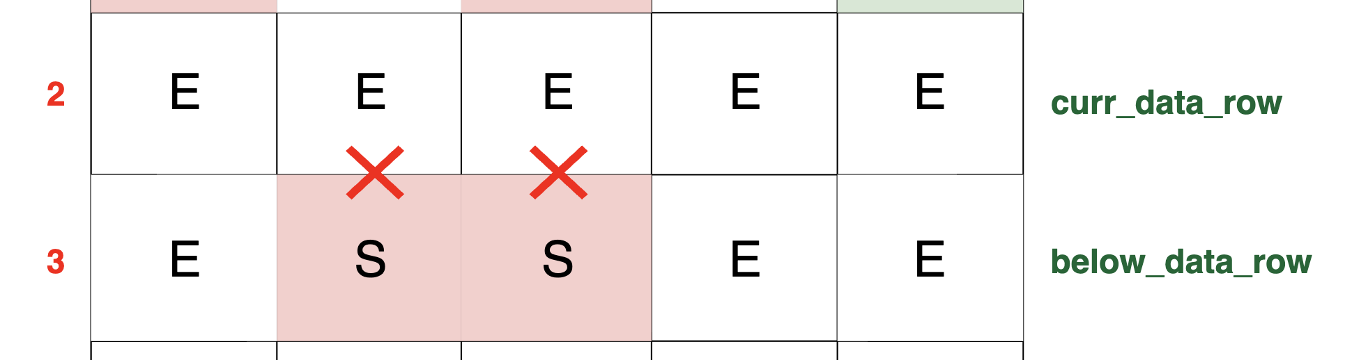
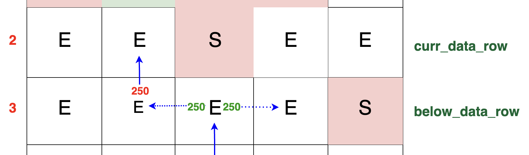
this cell because the block impedes any upward movement of packets. It simply means that there is no packet below because it's a switch. Observe in the diagram below that,
in the current row, there are two empty cells, and directly below these cells in the row below, there are blocks/switches (represented by S).
As a result, there is no packet flow into these specific cells in the current row, due to the obstructive presence of the switches in the row below:
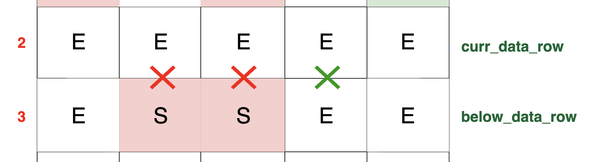
2) The Cell Below is Empty Without Any Packet (E): below_data_row[c] is 0 can also indicate that the below cell in the original grid is simply an empty cell
with no packet to flow upwards. Although the cell is not blocked and is capable of allowing packet flow, there is simply no packet in this particular cell to flow up to
curr_data_row[c]. Similarly, notice that the second to last cell (or column) in the current row also has no packet flow. This situation arises because the corresponding cell in
the row below doesn't contain any packet to flow upwards, as indicated by the value 0 in that cell, and the value E in the original grid's cell:
In either case, whether due to a block or the absence of a packet, below_data_row[c] == 0 effectively means there is no packet just below the current cell that can ascend.
Therefore, the algorithm continues to the next cell without making any changes to the packet amount in curr_data_row[c].
4) Packet Flow into Unblocked Cell
for r in range(rows - 2, -1, -1):
    # At each iteration, 'curr_data_row' is what we are trying to update
    # using values from 'below_data_row'.
    curr_data_row = [0] * cols
    for c in range(cols):
        # CASE 1:
        # There is no packet below to go up.
        if below_data_row[c] == 0:
            continue

        # CASE 2:
        # There is no switch in the current cell. There is no amplifier either.
        # Network packet can go directly up without splitting or amplifying.
        if server_grid[r][c] == 'E':
            curr_data_row[c] += below_data_row[c]

        ...
We have already examined Case-1, where the cell directly below has no packet to ascend (being either a switch or an empty cell). In Case-2, it's established
that the value of the cell directly below, indicated by below_data_row[c], is positive, suggesting that we have packets in the row below that want to move upward.
Moreover, server_grid[r][c] == 'E' signifies that the current cell is empty, which indicates that the packets in the cell below can flow upward.
Let's delve deeper into the code snippet:
# CASE 2:
# There is no switch in the current cell. There is no amplifier either.
# Network packet can go directly up without splitting or amplifying.
if server_grid[r][c] == 'E':
    curr_data_row[c] += below_data_row[c]
...
Here, the key operation is the condition if server_grid[r][c] == 'E'. This line crucially determines the state of the current cell. Any packet in the row below,
indicated by below_data_row[c], can simply move upward without obstruction since our current cell is empty.
When the condition server_grid[r][c] == 'E' is met (indicating an unblocked cell), the algorithm adds the packet amount from the cell directly below (below_data_row[c])
to curr_data_row[c].
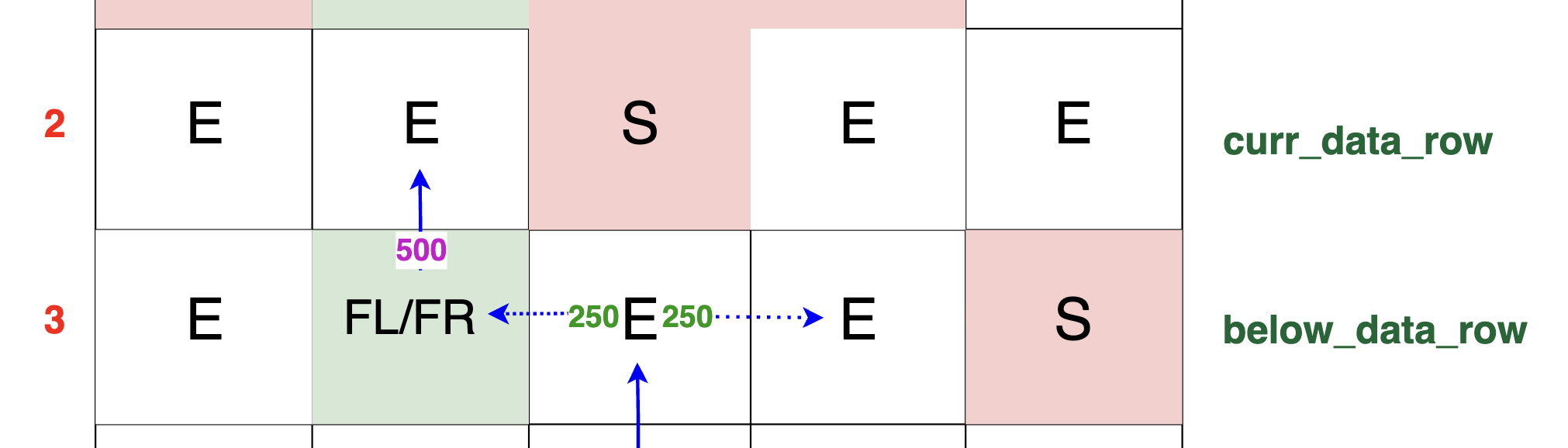
Below is a diagram illustrating the packet flow from the row below when the current cell (i.e., server_grid[r][c] == 'E') is empty:
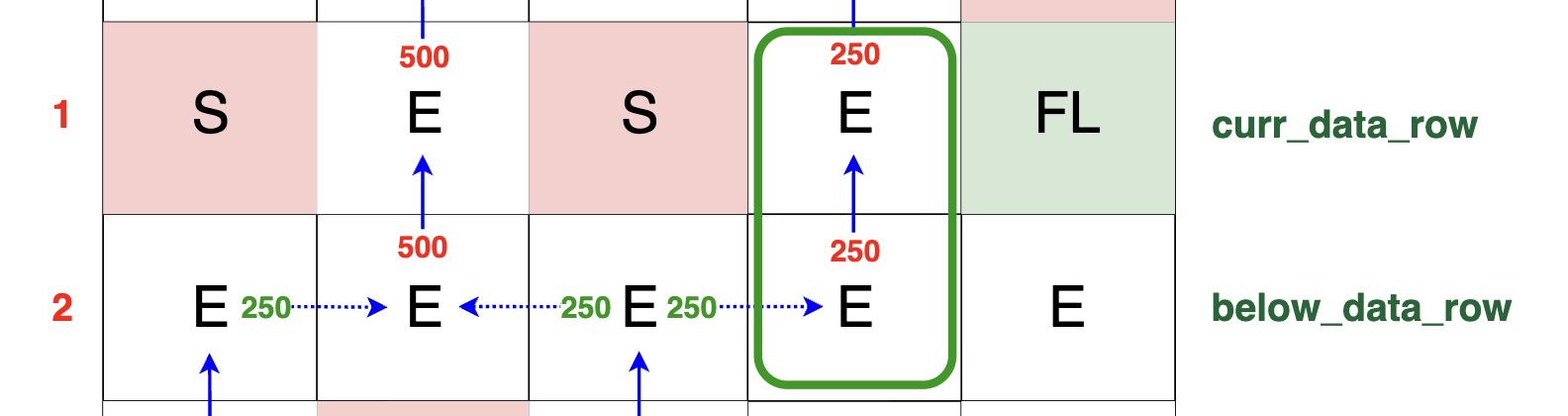
Observe the green highlighted rectangle in the diagram. It shows that the row below has 250 TB of the packets while the current cell's value is E (server_grid[r][c] == 'E').
This indicates that the current cell is empty and ready to receive the packets from below. This scenario corresponds to the operation curr_data_row[c] += 250, resulting in
curr_data_row[c] = 250.
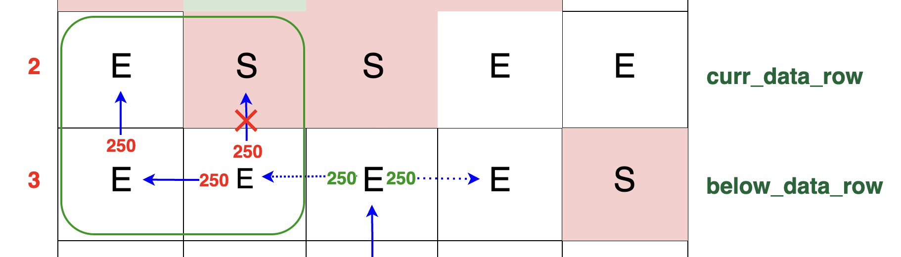
It's also possible that the current cell already contains some packets, indicated by a positive value. In this case, the process remains the same. We simply add the packet amount from below directly to our current cell:
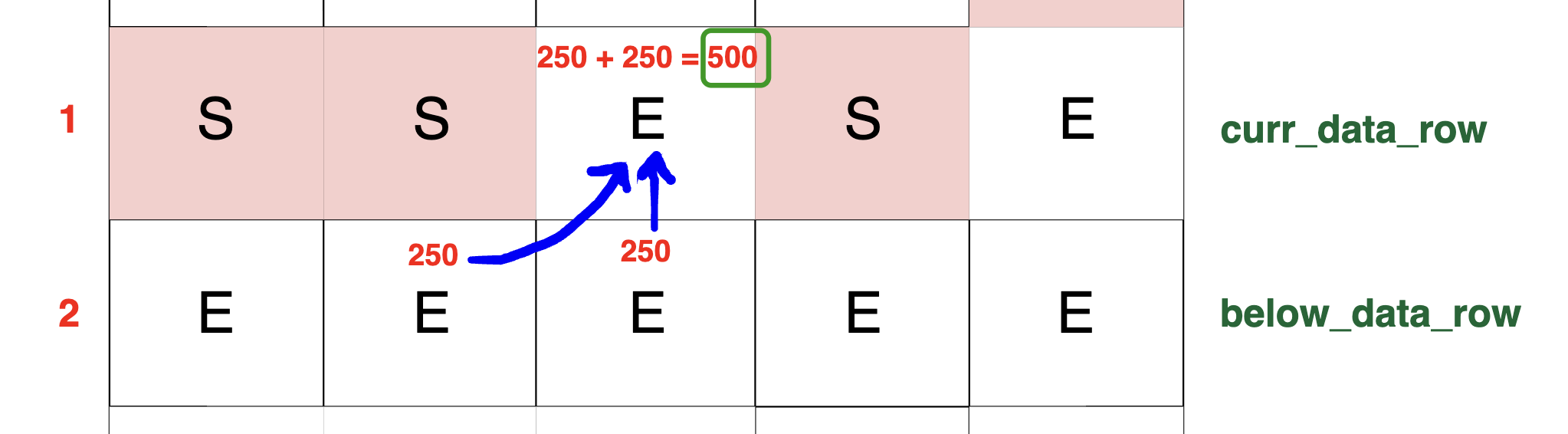
First, consider the cell in the row below that has 250 TB of the packets; these packets flow into our current cell because of the presence of blocks (S) above in current row.
When we focus on the current cell's turn (e.g., curr_data_row[c]), we observe that there are packets right above it as well, amounting to 250 TB. Therefore, we add this 250 to the
already existing packets in our cell, resulting in a combined total of 250 + 250 = 500 in our current cell.
5) Packet Flow into Amplifying Cell
Amplifying cells, represented by FL (amplifier left) and FR (amplifier right), have unique behaviors that not only amplify the data packets but also redirect them based on their predefined directions:
- FL (Amplifier Left): This cell multiplies the incoming data packet by a specified factor and attempts to redirect it to the left. If the left path is blocked, the packet moves upward.
- FR (Amplifier Right): This cell multiplies the incoming data packet by a specified factor and attempts to redirect it to the right. If the right path is blocked, the packet moves upward.
This is indicated by the code snippet below:
# CASE 3:
# There is an amplifier in the current cell. Based on the direction,
# the packet will move accordingly from 'below_data_row' to 'curr_data_row'.
elif server_grid[r][c] in ('FL', 'FR'):
    handle_amplifier(server_grid, curr_data_row, r, c, below_data_row[c], server_grid[r][c], amplifier_factor)
...
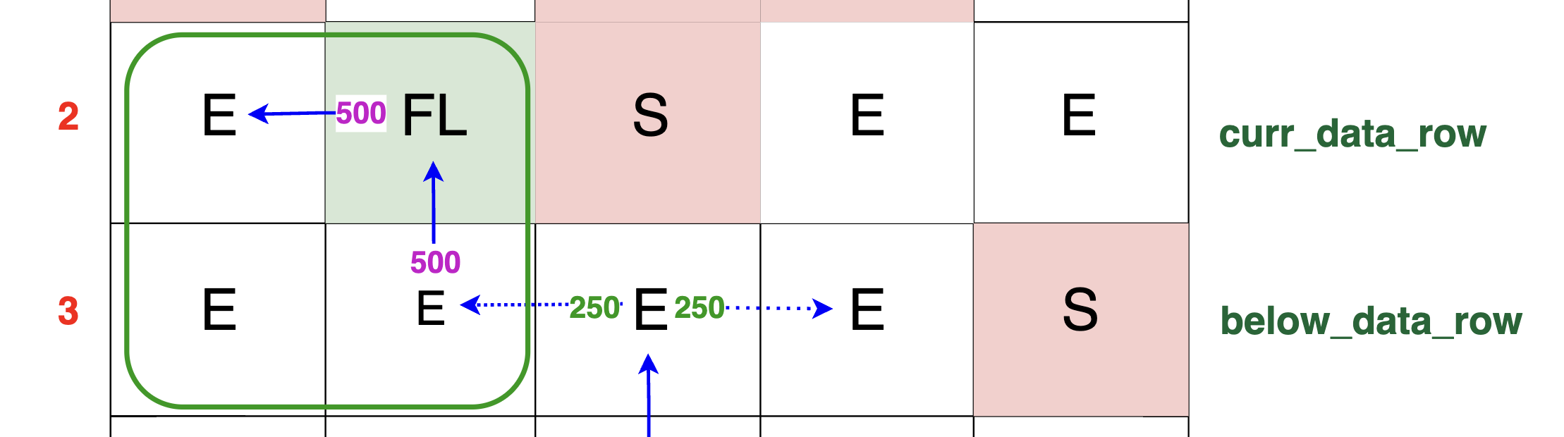
Below is a diagram illustrating the packet flow from the row below when the current cell (i.e.,server_grid[r][c] == 'FL')` is amplifier left:
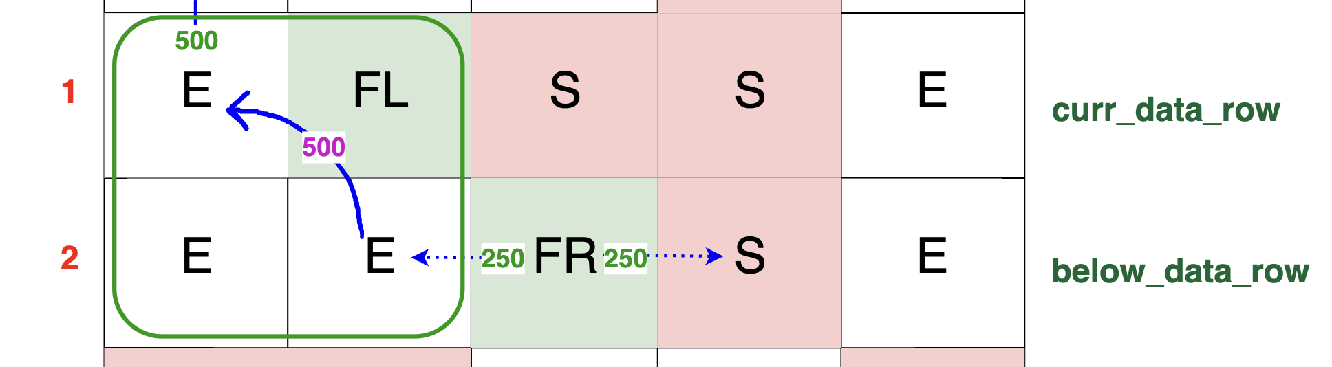
Observe that the packet arrives as 250 TB to the empty cell (E) and encounters a left amplifier in the current row
(i.e., server_grid[r][c] == 'FL'). This multiplies the existing packet by two, resulting in a packet of 500 TB, and redirects it to the left as
shown in the diagram. The packet was able to turn left because the (FL) cell has an empty cell (E) to its left. Now, let's look at the case where
the cell on its left is a block (S).
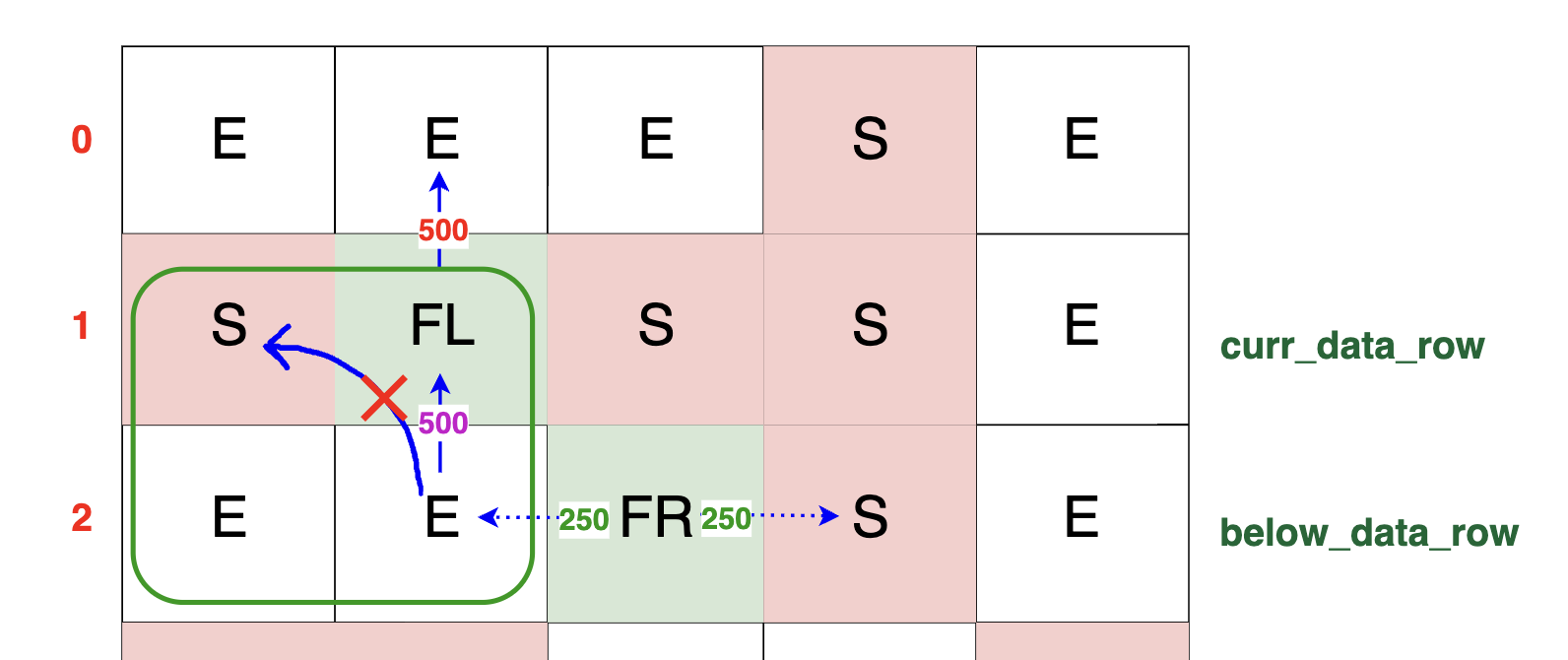
If the cell on its left were a block (S), then (FL) would only amplify the packet without redirecting it, essentially acting like an empty space (E):
This is all handled in our handle_amplifier method, which is called when the packet in the row below encounters an amplifier (FL) or (FR) in the
cell above, namely the current cell (i.e., server_grid[r][c]). Below is the code snippet:
# Helper method to amplify the network packet and potentially redirect it.
def handle_amplifier(server_grid, curr_data_row, r, c, data, direction, amplifier_factor):
    amplified_data = data * amplifier_factor
    curr_row_original = server_grid[r]
    # Amplify and try to move left.
    if direction == 'FL':
        # The cell on the left is not a blocker, so we can amplify and move there.
        if c > 0 and curr_row_original[c - 1] != 'S':
            curr_data_row[c - 1] += amplified_data
        # We are blocked on the left, so simply amplify and move upwards.
        else:
            curr_data_row[c] += amplified_data
    # Amplify and try to move right.
    elif direction == 'FR':
        # The cell on the right is not a blocker, so we can amplify and move there.
        if c < len(curr_data_row) - 1 and curr_row_original[c + 1] != 'S':
            curr_data_row[c + 1] += amplified_data
        # We are blocked on the right, so simply amplify and move upwards.
        else:
            curr_data_row[c] += amplified_data
...
As you can see, we first amplify the packet using the amplifier_factor. Then, based on the provided direction (FL or FR), we redirect the packet accordingly.
There are two possibilities:
1) Cell on the left (for FL) or cell on the right (for FR) is free (E): This is the scenario we have already discussed. If the cell to the left is free and the current cell is an (FL), we move the packet to the left. Similarly, if the cell to the right is free and the current cell is an (FR), we move the packet to the right. This is because the adjacent cell is empty (i.e., E). The code snippets below demonstrate this:
- For (FL), we update the cell to the left of the current cell:
curr_data_row[c - 1] += amplified_data. - For (FR), we update the cell to the right of the current cell:
curr_data_row[c + 1] += amplified_data.
# Amplify and try to move left.
if direction == 'FL':
    # The cell on the left is not a blocker, so we can amplify and move there.
    if c > 0 and curr_row_original[c - 1] != 'S':
        curr_data_row[c - 1] += amplified_data
    ...
# Amplify and try to move right.
elif direction == 'FR':
    # The cell on the right is not a blocker, so we can amplify and move there.
    if c < len(curr_data_row) - 1 and curr_row_original[c + 1] != 'S':
        curr_data_row[c + 1] += amplified_data
    ...
Our previous diagram illustrates this scenario for the left amplifier - (FL):
2) Cell on the left (for FL) or cell on the right (for FR) is a switch (S): In this scenario, the packet cannot be redirected to the left or right
because the adjacent cell is a switch (i.e., S). Instead, the amplifier simply amplifies the packet, and it continues to move upward, acting as if the current
cell were empty (i.e., E). The code snippets below demonstrate this behavior. We are updating the current cell, not its left or right: curr_data_row[c] += amplified_data.
# Helper method to amplify the network packet and potentially redirect it.
def handle_amplifier(server_grid, curr_data_row, r, c, data, direction, amplifier_factor):
    # Amplify and try to move left.
    if direction == 'FL':
        ...
        # We are blocked on the left, so simply amplify and move upwards.
        else:
            curr_data_row[c] += amplified_data

    # Amplify and try to move right.
    elif direction == 'FR':
        ...
        # We are blocked on the right, so simply amplify and move upwards.
        else:
            curr_data_row[c] += amplified_data
...
Our previous diagram illustrates this scenario for the left amplifier - FL as well:
Another case where FL or FR acts as an empty cell (i.e., E) is when they are located at the left or right corners of the grid, respectively.
In these situations, since there is no cell to the left of an FL or to the right of an FR, the packet simply moves upward after amplification.
This is also covered in the handle_amplifier method.
The last scenario occurs when the current cell is a switch: server_grid[r][c] == 'S'. In this case, our packet will be split to the left and to the right.
Below, we will examine both scenarios.
6) Managing Packet Split and Flow to the Left and Right
In this scenario, our algorithm encounters a switch in the current cell (server_grid[r][c] == 'S'), which has a value of S. This blockage necessitates the splitting of packets within
below_data_row[c]. The key idea here is to redirect the flow of these packets around the switch, splitting them equally to both the left and right.
Given that current cell - server_grid[r][c] - is a switch, we first split the packet coming from below:
# We have a switch ('S') in the current cell.
# Packet needs to be split in two directions: Left and Right before moving up.
else:
    halved_packet = below_data_row[c] / 2
    handle_split(server_grid, curr_data_row, r, c, halved_packet, amplifier_factor, 'left')
    handle_split(server_grid, curr_data_row, r, c, halved_packet, amplifier_factor, 'right')
...
Here, halved_packet calculates half of the packet's value from below_data_row[c]. This halved value will be distributed either to the left or right of the block,
wherever a clear path is available. Observe the diagram below for a visual help:
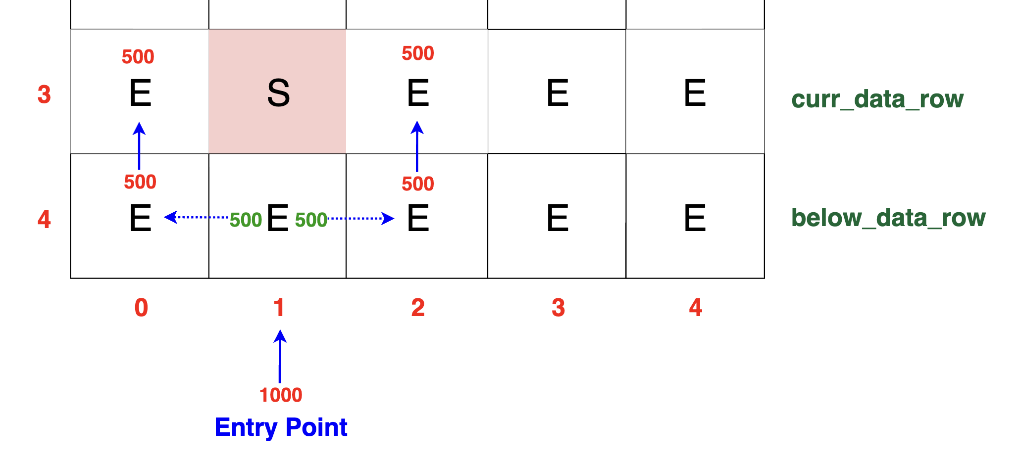
In the diagram above, both the left and right paths are unobstructed. Consequently, the packets will be evenly distributed, with 500 TB flowing to the left (curr_data_row[c - 1])
and 500 TB flowing to the right
(curr_data_row[c + 1]). This equal division ensures that the packet flow adapts efficiently around the block, utilizing available paths.
Now that we have grasped the concept of packet splitting, let's delve into the specific mechanics of how these packets flow in the left direction. The process for packet distribution in
the right direction is identical but adjusted for the opposite side. Below is our handle_split helper method, which splits the packet based on the provided direction:
# Case where there is a packet below, but the current cell has a block.
# Packet needs to be split in two directions: Left and Right.
# The direction is decided based on the 'direction' parameter's value.
def handle_split(server_grid, curr_data_row, r, c, halved_packet, amplifier_factor, direction):
    if direction == 'left':
        start, end, step = c - 1, -1, -1
    else:
        start, end, step = c + 1, len(curr_data_row), 1

    below_row_original = server_grid[r + 1]
    curr_row_original = server_grid[r]

    for idx in range(start, end, step):
        # Packet below is blocked by a cell on its direction.
        # Hence, it cannot go up.
        if below_row_original[idx] == 'S':
            break
        # The packet below is amplified by either 'FL' or 'FR',
        # Since the packet passes by this cell (e.g., the FL/FR is not above the packet),
        # there won't be any redirection.
        if below_row_original[idx] in ('FL', 'FR'):
            halved_packet *= amplifier_factor
            # Cell above is a blocker, continue in specified direction.
            if curr_row_original[idx] == 'S':
                continue
            # Cell above is an amplifier.
            if curr_row_original[idx] in ('FL', 'FR'):
                handle_amplifier(server_grid, curr_data_row, r, idx, halved_packet, curr_row_original[idx], amplifier_factor)
            # Cell above is an empty space, so we can move directly up.
            else:
                curr_data_row[idx] += halved_packet
            break
        # The cell below is an empty space.
        else:
            # Cell above is a blocker, continue in specified direction.
            if curr_row_original[idx] == 'S':
                continue
            # Cell above is an amplifier.
            if curr_row_original[idx] in ('FL', 'FR'):
                handle_amplifier(server_grid, curr_data_row, r, idx, halved_packet, curr_row_original[idx], amplifier_factor)
            # Cell above is an empty space, so we can move directly up.
            else:
                curr_data_row[idx] += halved_packet
            break
As you can see, based on the specified direction (left split or right split), we determine the boundaries of our iteration. This allows us to appropriately split the packet and direct it to either the left or the right while considering the constraints of the grid:
if direction == 'left':
    start, end, step = c - 1, -1, -1
else:
    start, end, step = c + 1, len(curr_data_row), 1
1) Avoiding Left-Side Blocks: The loop checks each cell to the left (left_idx = c - 1). If it encounters a block in below row (below_row_original[left_idx] == 'S'),
indicating that the packet cannot follow that path, the loop is terminated. The diagram below shows this example scenario:
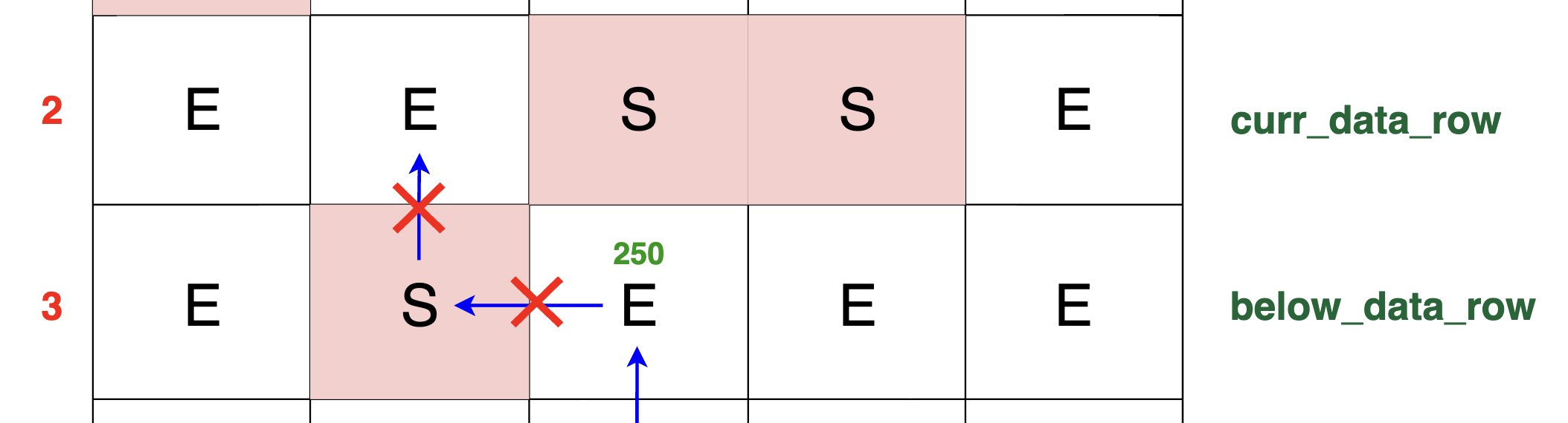
Given that there is a block on the left-hand side in below row (specifically, below_row_original[left_idx] == 'S'), the packets are prevented from ascending through the left path.
Consequently, this triggers a break in the loop, prompting the algorithm to cease exploring the left direction and instead proceed to evaluate the possibility of packet
flow in the right direction.
2) Finding an Open Path (FL or FR): When seeking a path for the split packet, the algorithm first ensures that the cell in the row below (below_row_original[left_idx]) is not a block.
If below_row_original[left_idx] != 'S', indicating there is no obstruction directly below, then below_row_original[left_idx] can be either (FL), (FR), or (E).
It then checks if the corresponding cell in the current row (curr_row_original[left_idx]) is unblocked
(curr_row_original[left_idx] != 'S').
When we split the packet due to the row above (curr_row[idx]) being a switch, and we encounter an FL or FR in our left direction while finding an open path, the FL or FR
cell does not affect the direction. Instead, it acts like an empty cell (E) but amplifies the packet. This means the packet continues in its original direction, either left or right,
while its value is increased by the amplifier factor.
Let's consider the case of FL or FR. In this case, the algorithm amplifies
halved_packet using halved_packet *= amplifier_factor.
Upon finding that the cell is unblocked (curr_row_original[left_idx]), the algorithm amplifies halved_packet using halved_packet *= amplifier_factor.
However, curr_row_original[left_idx] can also be any of (E), or (S) which will affect the path that the packet needs to follow. The code snippet below shows these possibilities:
In the code snippet below, we also consider the possibility of curr_row_original[left_idx] being (FL) or (FR). However, the question prompt
explicitly states that a column in the server_grid can only contain one (FL) or (FR). Since below_row_original[left_idx] is itself (FL)
or (FR), the cell above it - curr_row_original[left_idx] - can only be (E) or (S).
# The packet below is amplified by either 'FL' or 'FR',
# Since the packet passes by this cell (e.g., the FL/FR is not above the packet),
# there won't be any redirection.
if below_row_original[idx] in ('FL', 'FR'):
    halved_packet *= amplifier_factor
    # Cell above is a blocker, continue in specified direction.
    if curr_row_original[idx] == 'S':
        continue
    # Cell above is an amplifier.
    if curr_row_original[idx] in ('FL', 'FR'):
        handle_amplifier(server_grid, curr_data_row, r, idx, halved_packet, curr_row_original[idx], amplifier_factor)
    # Cell above is an empty space, so we can move directly up.
    else:
        curr_data_row[idx] += halved_packet
    break
If curr_row_original[left_idx] == 'S', meaning the cell above is a switch, then the packet continues to move left after being amplified. If there is no block in the left direction,
the packets traverse to the left until they find a viable path up to our current row. This movement is exemplified by the green rectangle in the diagram. The first unobstructed cell
in our current row on the left-hand side happens to be the very last cell. As clearly illustrated, the entire 500 TB of packets find their way up into this cell:
When below row contains packets to flow upwards, and the directly corresponding cell in current row is blocked, the algorithm implements a strategic redirection
of packets. It attempts to guide the flow towards the nearest unblocked cells in the current row, both to the left and the right side of the block. This approach ensures
that packets find the nearest available paths around the switch. This is where the next step comes in: decrementing left_idx for the left split and incrementing right_idx for the right split.
The boundaries and steps for idx are determined at the beginning of the method, as we previously discussed.
If curr_row_original[left_idx] == 'E', meaning the cell above is empty, then the packet simply moves upward into this cell after being amplified.
There is no obstruction, so the packet does not need to search for an alternative path. The packet continues its journey directly upward. The entire 500 TB of packets move up into this cell,
demonstrating a straightforward traversal when the cell above is empty:
3) Finding an Open Path (E): When seeking a path for the split packet, the algorithm first ensures that the cell in the row below (below_row_original[left_idx]) is not a block.
If below_row_original[left_idx] != 'S', indicating there is no obstruction directly below, then below_row_original[left_idx] can be either (E), (FL), or (FR). It then checks if
the corresponding cell in the current row (curr_row_original[left_idx]) is unblocked
(curr_row_original[left_idx] != 'S).
When we split the packet due to the row above (curr_row[idx]) being a switch, and we encounter an E in our left direction while finding an open path, the E cell simply allows the packet
to continue in its original direction without amplification. This means the packet continues in its original direction, either left or right, without any change in value.
If curr_row_original[left_idx] == 'S', meaning the cell above is a switch, then the packet continues to move left. If there is no block in the left direction,
the packets traverse to the left until they find a viable path down to our current row. This movement is exemplified by the green rectangle in the diagram. The first unobstructed cell
in our current row on the left-hand side happens to be the very last cell. As clearly illustrated, the entire 250 TB of packets find their way up into this cell:
If curr_row_original[left_idx] == 'E', meaning the cell above is empty, then the packet simply moves upward into this cell.
There is no obstruction, so the packet does not need to search for an alternative path. The packet continues its journey directly upward. The entire 250 TB of packets move up into this cell,
demonstrating a straightforward traversal when the cell above is empty:
If curr_row_original[left_idx] == 'FL', meaning the cell above is a left amplifier, then the packet is amplified and redirected to the left. The packet value is multiplied by the amplifier factor,
increasing its amount. If the left path is unblocked, the packet continues to move left. The entire 500 TB of packets, after amplification, will be directed leftward into the next cell,
demonstrating how the packet's path is influenced by an amplifier:
As discussed, this case is handled by our handle_amplifier function:
# Cell above is an amplifier.
if curr_row_original[idx] in ('FL', 'FR'):
    handle_amplifier(server_grid, curr_data_row, r, idx, halved_packet, curr_row_original[idx], amplifier_factor)
...
The case where curr_row_original[left_idx] == 'FR' is similar, except that we redirect the packet to the right if the path is clear. If the right cell is blocked,
the packet simply moves upward.
7) Update the Current Row to be the New Row Above
After processing the packet distribution for the current row, a critical step in our algorithm involves preparing for the next iteration.
This is achieved by updating below_data_row to reference curr_data_row:
# The updated current row will act as the `below_data_row` in the next iteration.
below_data_row = curr_data_row
This assignment ensures that the packets distributed in the current iteration (curr_data_row) become the basis for the next iteration.
Essentially, curr_data_row from the current step becomes below_data_row for the next step. By making curr_data_row the new below_data_row, the algorithm seamlessly transitions
from one row to the next, maintaining the continuity of packet flow across rows without any loss of data or context.
We apply the same logic of packet flow and distribution based on the updated data from the previous cycle.
Complexity Analysis
Time Complexity: O(c² × r), where c represents the number of columns (cells) in each row, and r represents the number of rows within the grid.
Explanation:
1) Iterating Through Each Row
- The algorithm iterates through each row of the grid, updating each row based on the row below, continuing until the packet percentages in the first row (the exit row) are calculated. This contributes to a O(r) time complexity, where r represents the number of rows within the grid.
2) Processing Each Cell within a Row
- Within each row, every cell is processed, which contributes to a O(c) time complexity, where c represents the number of cells/columns within a row. However, note that for some cells, especially those that encounter a switch/block, the packet may need to be split and redirected. This results in examining adjacent cells, potentially leading to nested iterations over the columns in the worst-case scenario, particularly when trying to find alternative paths around blocks.
3) Checking the Left and Right Directions for Each Cell in the Row
- For each blocked cell, the algorithm checks both left and right directions to find open paths. In the worst case, this could involve scanning up to c cells in each direction, hence contributing to the quadratic component in the time complexity, O(c²). Multiplied by the number of rows r, the overall time complexity in the worst-case scenario can amount to O(c² × r).
Combining these steps, the overall time complexity of the algorithm would be O(c² × r).
The average time complexity is in fact O(c x r) because the algorithm iterates linearly through each column of every row, processing packet flows and redirections. Redirections due to blocks generally do not involve re-checking every column but are limited to nearby open cells, significantly reducing the potential for quadratic behavior. Thus, most operations are constrained to direct interactions within or near the immediate column, aligning the complexity more closely with the number of rows and columns rather than their square.
Space Complexity: O(c): The algorithm uses additional arrays below_data_row and curr_data_row, each of length equal to the number of columns. These arrays are used to store the packet data for the current and the row below, respectively. Thus, the space complexity is linear in terms of the number of columns.
Below is the coding solution for the algorithm we've just explored:
# O(c^2 * r) time | O(c) space
def data_packet_distribution(server_grid, entry_point, data_amount, amplifier_factor):
    rows = len(server_grid)
    cols = len(server_grid[0])

    # Last row will have a cell (entry) from which
    # data packet will move up. Hence, we update the cell value to 'data_amount'.
    below_data_row = [0] * cols
    below_data_row[entry_point] = data_amount

    for r in range(rows - 2, -1, -1):
        # At each iteration, 'curr_data_row' is what we are trying to update
        # using values from 'below_data_row'.
        curr_data_row = [0] * cols
        for c in range(cols):
            # There is no packet below to go up.
            if below_data_row[c] == 0:
                continue
            # There is no switch in the current cell. There is no amplifier either.
            # Network packet can go directly up without splitting or amplifying.
            if server_grid[r][c] == 'E':
                curr_data_row[c] += below_data_row[c]
            # There is an amplifier in the current cell. Based on the direction,
            # the packet will move accordingly from 'below_data_row' to 'curr_data_row'.
            elif server_grid[r][c] in ('FL', 'FR'):
                handle_amplifier(server_grid, curr_data_row, r, c, below_data_row[c], server_grid[r][c], amplifier_factor)
            # We have a switch ('S') in the current cell.
            # Packet needs to be split in two directions: Left and Right before moving up.
            else:
                halved_packet = below_data_row[c] / 2
                handle_split(server_grid, curr_data_row, r, c, halved_packet, amplifier_factor, 'left')
                handle_split(server_grid, curr_data_row, r, c, halved_packet, amplifier_factor, 'right')

        below_data_row = curr_data_row

    total_data = sum(below_data_row)
    return [total_data, below_data_row]

# Helper method to amplify the network packet and potentially redirect it.
def handle_amplifier(server_grid, curr_data_row, r, c, data, direction, amplifier_factor):
    amplified_data = data * amplifier_factor
    curr_row_original = server_grid[r]
    # Amplify and try to move left.
    if direction == 'FL':
        # The cell on the left is not a blocker, so we can amplify and move there.
        if c > 0 and curr_row_original[c - 1] != 'S':
            curr_data_row[c - 1] += amplified_data
        # We are blocked on the left, so simply amplify and move upwards.
        else:
            curr_data_row[c] += amplified_data
    # Amplify and try to move right.
    elif direction == 'FR':
        # The cell on the right is not a blocker, so we can amplify and move there.
        if c < len(curr_data_row) - 1 and curr_row_original[c + 1] != 'S':
            curr_data_row[c + 1] += amplified_data
        # We are blocked on the right, so simply amplify and move upwards.
        else:
            curr_data_row[c] += amplified_data

# Case where there is a packet below, but the current cell has a block.
# Packet needs to be split in two directions: Left and Right.
# The direction is decided based on the 'direction' parameter's value.
def handle_split(server_grid, curr_data_row, r, c, halved_packet, amplifier_factor, direction):
    if direction == 'left':
        start, end, step = c - 1, -1, -1
    else:
        start, end, step = c + 1, len(curr_data_row), 1

    below_row_original = server_grid[r + 1]
    curr_row_original = server_grid[r]

    for idx in range(start, end, step):
        # Packet below is blocked by a cell on its direction.
        # Hence, it cannot go up.
        if below_row_original[idx] == 'S':
            break
        # The packet below is amplified by either 'FL' or 'FR',
        # Since the packet passes by this cell (e.g., the FL/FR is not above the packet),
        # there won't be any redirection.
        if below_row_original[idx] in ('FL', 'FR'):
            halved_packet *= amplifier_factor
            # Cell above is a blocker, continue in specified direction.
            if curr_row_original[idx] == 'S':
                continue
            # Cell above is an amplifier.
            if curr_row_original[idx] in ('FL', 'FR'):
                handle_amplifier(server_grid, curr_data_row, r, idx, halved_packet, curr_row_original[idx], amplifier_factor)
            # Cell above is an empty space, so we can move directly up.
            else:
                curr_data_row[idx] += halved_packet
            break
        # The cell below is an empty space.
        else:
            # Cell above is a blocker, continue in specified direction.
            if curr_row_original[idx] == 'S':
                continue
            # Cell above is an amplifier.
            if curr_row_original[idx] in ('FL', 'FR'):
                handle_amplifier(server_grid, curr_data_row, r, idx, halved_packet, curr_row_original[idx], amplifier_factor)
            # Cell above is an empty space, so we can move directly up.
            else:
                curr_data_row[idx] += halved_packet
            break
Final Notes
We believe this question has been asked frequently by Google in recent interviews! This server load distribution problem is a focal topic in recent technical discussions at Google, underscoring the essential role of efficient data flow management within network infrastructures. This is also one of the most challenging questions Google has been asking recently, and the provided time for solving it is accordingly longer than usual. From our understanding, the allotted time is 60 minutes.
We believe solving this particular question is crucial if you're interviewing with Google soon. It has been frequently asked in recent interviews, and understanding its solution will aid you in addressing similar problems that Google might ask. Efficient network packet management is not just crucial, it's central to maintaining the high-performance standards expected at Google. Understanding and optimizing how data moves across networks, and integrating this with algorithmic solutions, are indispensable skills looked for by Google. Here are several insights and strategies to consider from this exercise:
1) Understanding Network Flow: Mastery of how data or packets navigate through a network is essential. This question provides a clear visualization of dynamic routing decisions: core to network management at Google.
2) Handling Edge Cases: The presence of numerous edge cases makes this question particularly challenging. Solving it perfectly is not the primary focus for the interviewer. The chances of fully solving it within the allotted 90 minutes are low. What the interviewer wants to see is your thought process, how you approach problem-solving, and your ability to communicate effectively with a fellow teammate.
3) Adaptability to Network Dynamics: The problem demonstrates how to handle dynamic conditions akin to real-life scenarios at Google, where packet routing must adapt due to blockages or network traffic.
4) Efficient Algorithm Design: Utilizing a systematic approach to simulate packet distribution and efficiently managing obstacles using directional splits showcases your capability to devise solutions that are both effective and efficient, a quality highly valued at Google.
5) Complexity Analysis: Discussing the time and space complexities is critical in environments like Google's, where scalability and performance are pivotal. This solution highlights a balance between computational efficiency and operational simplicity.
6) Practical Relevance: Designed on a grid-based model, this scenario mirrors network topologies used in Google's data centers, making it highly relevant to understanding routing algorithms in networking contexts.
7) Innovative Problem Solving: This solution reflects the innovative problem-solving skills Google looks for—critical in optimizing network performance and reducing operational costs in its vast tech infrastructure.
8) Communication of Complex Ideas: Demonstrating your approach in solving complex problems effectively is crucial at Google, where you often need to collaborate with cross-functional teams that rely on clear and concise communication.
9) Real-World Application: While the problem is theoretical, the principles directly apply to real-world scenarios at Google, where efficient data routing is paramount to maintaining robust network services and infrastructure.
Preparing for a role at Google means not only showcasing your technical expertise but also demonstrating how these skills can lead to practical improvements within such a sophisticated and dynamic environment. That's why Google has recently incorporated this question into their interviews. Mastering the approach and demonstrating clear problem-solving methodology will significantly enhance your performance during the interview process.
Step into this challenge with confidence, knowing that your ability to navigate such complex scenarios will set you apart as a candidate ready to contribute effectively to Google's ambitious projects. We hope that you will see this question in your interview and remember us! Good luck!