Q1 - Hub Site Selection for Amazon Prime
We believe a variation of this interview question has recently been asked by Amazon to full-time junior software engineering candidates.
In the dynamic world of Amazon's operations, the positioning of a Prime distribution hub is a pivotal decision that impacts delivery speed, operational efficiency, and ultimately customer satisfaction. As a Logistics Software Engineer, you are entrusted with the critical task of identifying the most strategically located site for a new hub, ensuring Amazon continues to deliver products with the swiftness and efficiency that customers expect.
The challenge before you involves evaluating potential hub sites along a vital commercial corridor. Each site is a candidate for the new hub and offers varying access to four key logistical components: highways for ground transport, cargo airports for global shipping, warehouses for stock, and postal centers for mail distribution.
Your task is to create a function that receives a list of these sites and Amazon's requirements for logistical services. Each site in
the list includes values indicating the presence 1 or absence 0 of each logistical asset, such as highways,
cargo airports, or postal centers. Additionally, each requirement has an associated weight, acting as a penalty factor that increases the distance if a required service is not present at a site.
For instance, if a requirement has a high weight, the distance to the nearest site with that requirement will be multiplied by this weight, indicating its importance.
Your function should assess these sites to determine which one reduces the maximum distance to all necessary services and return the index of this optimal site. Selecting the right site is a strategic move that will significantly enhance the efficiency of Amazon Prime's logistics network.
The solution is expected to operate with a time complexity of no more than O(s * r), where s represents the number of candidate hub sites, and r represents the number of the distinct requirements.
Example
Input:
sites = [
  {
    "highway": 1,
    "cargo airport": 1,
    "warehouse": 1,
    "postal center": 0
  },
  {
    "highway": 0,
    "cargo airport": 1,
    "warehouse": 0,
    "postal center": 0
  },
  {
    "highway": 0,
    "cargo airport": 0,
    "warehouse": 1,
    "postal center": 0
  },
  {
    "highway": 0,
    "cargo airport": 1,
    "warehouse": 0,
    "postal center": 1
  },
  {
    "highway": 1,
    "cargo airport": 1,
    "warehouse": 0,
    "postal center": 0
  }
]

reqs = ["highway", "cargo airport", "warehouse", "postal center"]
weights = [2, 5, 3, 4]

Output:
3 // The site at idx=3 is the most optimal one.

Explanation:
Site at Index 0:
- Meets: highway (d=0), cargo airport (d=0), warehouse (d=0)
- Does not meet: postal center (d=3*4=12)
  Site-0 has all the required logistical components besides a postal center,
  which has a weight of 4.
  The nearest postal center is at Site-3, hence the distance is 3. Since its weight is 4,
  the actual distance is (d=12).
  This results in a max distance of `12` for Site-0.

Site at Index 1:
- Meets: cargo airport (d=0)
- Does not meet: highway (d=1*2=2), warehouse (d=1*3=3), postal center (d=2*4=8)
  Site-1 lacks a highway, warehouse and a postal center.
  The closest highway passes by Site-0, hence its distance to Site-1 is d=1*2=2.
  The closest warehouse is at either of Site-0 or Site-2, hence its distance to Site-1 is d=1*3=3.
  Finally, the closest postal center is at Site-3, hence its distance to Site-1 is d=2*4=8.
  This results in a max distance of `8` for Site-1.

Site at Index 2:
- Meets: warehouse (d=0)
- Does not meet: highway (d=2*2=4), cargo airport (d=1*5=5), postal center (d=1*4=4)
  Site-2 lacks a highway, cargo airport and a postal center.
  The closest highway passes by Site-0 or Site-4, hence its distance to Site-2 is d=2*2=4.
  The closest cargo airport is at Site-1 or Site-3, hence its distance to Site-2 is d=1*5=5.
  Finally, the closest postal center is at Site-3, hence its distance to Site-2 is d=1*4=4.
  This results in a max distance of `5` for Site-2.

Site at Index 3 [Optimal Site]:
- Meets: cargo airport (d=0), postal center (d=0)
- Does not meet: highway (d=1*2=2), warehouse (d=1*3=3)
  Site-3 lacks a highway and a warehouse.
  The closest highway passes by Site-4, hence its distance to Site-3 is d=1*2=2.
  The closest warehouse is at Site-2, hence its distance to Site-3 is d=1*3=3.
  This results in a max distance of `3` for Site-3.

Site at Index 4:
- Meets: highway (d=0), cargo airport (d=0)
- Does not meet: warehouse (d=2*3=6), postal center (d=1*4=4)
  Site-4 lacks a warehouse and a postal center.
  The closest warehouse is at Site-2, hence its distance to Site-4 is d=2*3=6.
  The closest postal center is at Site-3, hence its distance to Site-4 is d=1*4=4.
  This results in a max distance of `6` for Site-4.
Solution 1 (For intuition only - Not Accepted in the Interview)
We'll start by delving into a more intuitive method for solving this problem. Think for a moment: What's the most straightforward approach that springs to mind? It likely involves iterating through each site. At every site, we focus on a specific requirement—say, a highway—and search for the nearest site equipped with this logistical feature. We then measure the distance between our current site and this neighboring site with the required component. This process is repeated for each requirement to calculate a site's overall value. Once we've assessed the value of each site, our goal becomes clear: select the site that offers the shortest distance to all necessary logistical components.
Remember, when calculating a site's overall distance to all required logistical components, we specifically consider the maximum distance from that site to any single requirement. This maximum distance determines the site's overall proximity to the necessary services.
1) Iterate through all the Sites
Imagine walking through each site on the map. For each stop, we're asking: How far is the nearest highway?
The closest cargo airport? Warehouse? Postal center? But here's the twist - we're most interested in the furthest
of these services. Why? Because a hub is only as good as its farthest essential service. It's like making sure you're
not just near a highway but also not too far from a postal center. Check out the code snippet below. The variable
distance_to_reqs represents the overall value of a site, which is essentially the maximum distance from that site to
any of the specified requirements.
Iterating through the Sites
# Distance of the site with the minimum distance to the requirements.
min_site_distance = float('inf')
# The site idx with the minimum distance to the requirements.
min_distance_site_idx = 0
for i in range(len(sites)):
    # Current site's distance to the requirements (we take the max distance among the requirements).
    distance_to_reqs = float('-inf')
    for req_idx, req in enumerate(requirements):
        # Find the minimum distance from "site[i]" to the "req".
        min_req_distance = float('inf')
2) Iterate through all Requirements for each Site
As we scan each site, there's a step where we zoom in on every single requirement. It's not just about finding the furthest service overall but first identifying the closest instance of each required service. Here's how we do it: For each requirement at a site, say a highway or a postal center, we loop through all other sites to find the nearest one that offers this service. This step is like pinpointing the closest grocery store or gas station on a road trip. You can see this in the code snippet below:
Evaluating Sites against each other
for i in range(len(sites)):
    # Current site's distance to the requirements (we take the max distance among the requirements).
    distance_to_reqs = float('-inf')
    for req_idx, req in enumerate(requirements):
        # Find the minimum distance from "site[i]" to the "req".
        min_req_distance = float('inf')
        for j in range(len(sites)):
            # If the site[j] contains the "req", it may be the closest such site.
            if sites[j][req] == 1:
                min_req_distance = min(min_req_distance, abs(j - i) * weights[req_idx])
In this part of the code, we're evaluating each site j (other sites) to see if it has the required service req.
If it does, we calculate the distance from our current site i to this site j. We're continually updating
min_req_distance to hold the shortest distance found for this requirement.
Additionally, note the weight factor: each requirement's distance is multiplied by its associated weight (weights[req_idx]). This weight acts as a penalty factor, emphasizing
the importance of certain services over others. For instance, a higher weight increases the effective distance, prioritizing sites that minimize this weighted distance.
In our Example, cargo airport has a weight of 5, emphasizing its importance for selecting the optimal site for Amazon.
By determining the closest distances for individual requirements first, we set the stage for the next crucial step - finding the maximum distance. This detailed groundwork ensures that our final choice of site is not just good in one aspect but optimally positioned in all respects.
3) Assessing Overall Site Value
Evaluation of a Site's Value
for i in range(len(sites)):
    # Current site's distance to the requirements (we take the max distance among the requirements).
    distance_to_reqs = float('-inf')
    for req_idx, req in enumerate(requirements):
        # Find the minimum distance from "site[i]" to the "req".
        min_req_distance = float('inf')
        for j in range(len(sites)):
            # If the site[j] contains the "req", it may be the closest such site.
            if sites[j][req] == 1:
                min_req_distance = min(min_req_distance, abs(j - i) * weights[req_idx])
        # What matters is the maximum distance from "site[i]" to any of the requirements.
        # That 'max' value determines the value of the site for Amazon.
        distance_to_reqs = max(distance_to_reqs, min_req_distance)
Look at the last line in the above code snippet. After looping through each requirement and finding the nearest match,
we arrive at a critical juncture. We've got min_req_distance for each requirement, which is the shortest distance
from our current site i to a site that fulfills this specific requirement. We've explained this in the previous section.
We're not just content with these minimum distances. We want the maximum among these minimums. Why?
Because this maximum distance tells us how far the farthest essential service is from our site. Think of it as assessing
the worst-case scenario for an Amazon worker at this site. Sure, they might be close to a warehouse, but what if the nearest
postal center is quite far? This maximum distance will be the deciding factor.
The line of code distance_to_reqs = max(distance_to_reqs, min_req_distance) does exactly that. For each requirement,
it checks if min_req_distance is greater than our current distance_to_reqs (which is initially set to a very low value).
If it is, then distance_to_reqs gets updated. Essentially, by the end of checking all requirements, distance_to_reqs holds
the greatest of the minimum distances for this site.
4) Looking for the Optimal Site
Finding the Optimal Site
for i in range(len(sites)):
    # Current site's distance to the requirements (we take the max distance among the requirements).
    distance_to_reqs = float('-inf')
    for req_idx, req in enumerate(requirements):
        # Find the minimum distance from "site[i]" to the "req".
        min_req_distance = float('inf')
        for j in range(len(sites)):
            # If the site[j] contains the "req", it may be the closest such site.
            if sites[j][req] == 1:
                min_req_distance = min(min_req_distance, abs(j - i) * weights[req_idx])
        # What matters is the maximum distance from "site[i]" to any of the requirements.
        # That 'max' value determines the value of the site for Amazon.
        distance_to_reqs = max(distance_to_reqs, min_req_distance)
    # Check if we found a site with the minimum "max_distance" to the requirements.
    if distance_to_reqs < min_site_distance:
        min_site_distance = distance_to_reqs
        min_distance_site_idx = i
Now observe the last part of the code snippet above (e.g., if statement). With each site's maximum distance
determined, the next step is to find the best one: The aim is to identify the site with the smallest 'maximum distance'
among all sites. This site is the most strategically located in terms of overall accessibility to the required services
for Amazon.
Distance Comparison
# Check if we found a site with the minimum "max_distance" to the requirements.
if distance_to_reqs < min_site_distance:
    min_site_distance = distance_to_reqs
    min_distance_site_idx = i
By the end of this process, we have min_distance_site_idx, the index of the site that best meets Amazon Prime's logistical
requirements, embodying a balance of accessibility across all services. This approach ensures that the selected site isn't
just adequate but optimal for efficient operations and swift deliveries.
Complexity Analysis
-
Time Complexity: O(s² × r), where s represents the number of sites, and r represents the number of different requirements to be checked for each site.
Explanation:
-
Loop through each site
- For every site i in the list of sites, we initiate a nested process to evaluate its suitability. This first loop runs s times, where s is the total number of sites.
-
Evaluate each requirement
- Within each site iteration, we then loop through all requirements r. Each requirement must be checked against all other sites to determine the closest one meeting that requirement. This adds another r iterations.
-
Find the closest site for each requirement
- For each requirement, we loop through all s sites again to find the closest site that meets the requirement. This introduces another s iterations.
Combining these loops, the total time complexity is O(s² × r).
-
-
Space Complexity: O(1). The algorithm uses a constant amount of extra space. We only use a few variables to keep track of distances and indices, and the amount of space required does not scale with the size of the input.
This solution is certainly viable and would be partially acceptable. However, the optimal solution we're aiming for should ideally have a time complexity of O(s * r). As evident, this target complexity is a factor of s faster in runtime compared to the solution outlined above, (O(s2 * r)) making it significantly more efficient for larger datasets. However, as we'll discover later, achieving this more efficient time complexity comes with a trade-off: we need to slightly compromise our ideal space complexity of O(1).
Below is the coding solution for the algorithm we've just explored. In the next section, we will go through the expected solution with a better time complexity:
# O(s^2 * r) time | O(1) space
def optimal_site_search(sites, requirements, weights):
    # Distance of the site with the minimum distance to the requirements.
    min_site_distance = float('inf')
    # The site idx with the minimum distance to the requirements.
    min_distance_site_idx = 0
    for i in range(len(sites)):
        # Current site's distance to the requirements (we take the max distance among the requirements).
        distance_to_reqs = float('-inf')
        for req_idx, req in enumerate(requirements):
            # Find the minimum distance from "site[i]" to the "req".
            min_req_distance = float('inf')
            for j in range(len(sites)):
                # If the site[j] contains the "req", it may be the closest such site.
                if sites[j][req] == 1:
                    min_req_distance = min(min_req_distance, abs(j - i) * weights[req_idx])
            # What matters is the maximum distance from "site[i]" to any of the requirements.
            # That 'max' value determines the value of the site for Amazon.
            distance_to_reqs = max(distance_to_reqs, min_req_distance)
        # Check if we found a site with the minimum "max_distance" to the requirements.
        if distance_to_reqs < min_site_distance:
            min_site_distance = distance_to_reqs
            min_distance_site_idx = i

    return min_distance_site_idx
Solution 2 (Optimal Solution)
While Solution 1 presents a solid and comprehensive method for solving the problem, it is not without its challenges.
Coming up with such a solution already requires a deep understanding of the problem and the ability to handle complex nested loops.
Although it's a good solution in its own right, it falls short of meeting the ideal time complexity of O(s * r), a requirement
that often arises in technical interviews for roles demanding high efficiency in algorithmic solutions. However, keep in mind that
by implementing the first solution, you will already be ahead of 80% of the candidates!
Recognizing the need to align with these stringent performance constraints, we transition to Solution 2. This advanced solution significantly enhances time efficiency by reducing redundant computations, fitting neatly within the desired complexity boundary. However, this improvement in time efficiency comes with a trade-off in terms of space complexity.
It's essential to discuss these trade-offs with interviewers. Amazon values candidates who not only come up with efficient solutions but also understand and can articulate the implications of their design choices. Demonstrating this level of insight shows a deeper understanding of software engineering principles and the ability to balance different factors, such as time and space complexity, to arrive at the most effective solution for a given problem.
By presenting Solution 2 and discussing its trade-offs, you exhibit not only problem-solving skills but also a thoughtful consideration of real-world constraints and resources, a quality highly regarded in Amazon's technical interview process.
After reviewing Solution 1, an intuitive approach with a time complexity of O(s² * r), we turn our attention to Solution 2.
The key question here is: How do we improve the algorithm to reduce the complexity from O(s² * r) to the more efficient O(s * r)?
In Solution 1, the nested loop structure, where we compare each site with every other site for each requirement, contributes to the quadratic time complexity. Essentially, we're doing a lot of repeated work:
Nested loops within Solution 1
for i in range(len(sites)):
    # Current site's distance to the requirements (we take the max distance among the requirements).
    distance_to_reqs = float('-inf')
    for req_idx, req in enumerate(requirements):
        # Find the minimum distance from "site[i]" to the "req".
        min_req_distance = float('inf')
        for j in range(len(sites)):
            # If the site[j] contains the "req", it may be the closest such site.
            if sites[j][req] == 1:
                min_req_distance = min(min_req_distance, abs(j - i) * weights[req_idx])
        # What matters is the maximum distance from "site[i]" to any of the requirements.
        # That 'max' value determines the value of the site for Amazon.
        distance_to_reqs = max(distance_to_reqs, min_req_distance)
    # Check if we found a site with the minimum "max_distance" to the requirements.
    if distance_to_reqs < min_site_distance:
        min_site_distance = distance_to_reqs
        min_distance_site_idx = i
To optimize, we need to eliminate one layer of this iteration. But how? Solution 2 introduces a significant enhancement by pre-computing and storing the nearest distances of each requirement for every site. This way, instead of recalculating distances for each site and requirement pair, we refer to these pre-computed values. It's like creating a reference guide that quickly tells us how far each service is from any given site.
This approach removes the need for one of the inner loops that iterated over all sites for each requirement at every site,
thus reducing the time complexity to O(s * r). However, this improvement comes with a trade-off in space complexity,
which now increases to O(s * r).
1) Pre-Computing the Distance from each Site to each Requirement
Pre-Computation of distances to each Requirement
# (r x s) array containing the minimum distance from each site to each requirement.
# e.g., min_distances_from_sites[r][s] ==> minimum distance from site 's' to req 'r'.
min_distances_from_sites = []
for req_idx, req in enumerate(requirements):
    # Each iteration generates an array containing the min distance of each site to
    # the specific 'req' in the iteration.
    min_distances_from_sites.append(calculate_min_distances(sites, req, weights[req_idx]))
The first step is to create a 2D array (r x s), where each row corresponds to a specific requirement (like a highway or a postal
center), and each column represents a site. The element at position (i, j) in this array will store the minimum distance from
site j to the nearest site fulfilling requirement i. This part is done by the above code snippet.
The challenge lies in how to fill this matrix efficiently, e.g., calculate_min_distances(sites, req, weights[req_idx]) method.
Observe the code snippet below. You can see that we pre-compute the minimum distance between each site and a specific requirement. To achieve this we are doing 1) Left-to-Right Scan, and then 2) Right-to-Left Scan to update the values.
This method will be called for each requirement, and for each, it will return a row of the 2D array containing the shortest distances from every site to the nearest site that fulfills this specific requirement. For instance, if we're considering the requirement "highway", the method will produce a row in which each entry corresponds to a site, and the value at each entry represents the minimum distance from that site to the nearest site with a highway.
Calculating the Minimum Distance of a Site to a Requirement
# O(s) time | O(s) space
# Helper function to calculate the min distance of each site to a particular req.
# We do a Left-to-Right and then Right-to-Left iterations to update the values in O(s) time.
def calculate_min_distances(sites, req, weight):
    min_distances_to_req = [float('inf')] * len(sites)
    site_with_min_dist_idx = float('inf')
    # Scan the min distances from Left to Right.
    for i in range(len(sites)):
        if sites[i][req] == 1:
            site_with_min_dist_idx = i
        min_distances_to_req[i] = abs(i - site_with_min_dist_idx) * weight

    # Update the min distances by scanning from Right to Left.
    for j in range(len(sites) - 1, -1, -1):
        if sites[j][req] == 1:
            site_with_min_dist_idx = j
        min_distances_to_req[j] = min(min_distances_to_req[j],
                                      abs(j - site_with_min_dist_idx) * weight)

    return min_distances_to_req
-
Left-to-Right Scan: We start by scanning each row of the matrix from left to right. As we move, we keep track of the nearest site (up to that point) which fulfills the current requirement. This helps us update the minimum distance for each site on the go.
-
Right-to-Left Scan: After completing the left-to-right scan, we reverse our direction. This time, we scan from right to left, updating the minimum distances with any closer sites we find in this direction. This dual-scan approach ensures that each site's minimum distance to a requirement is accurately computed considering sites on both sides.
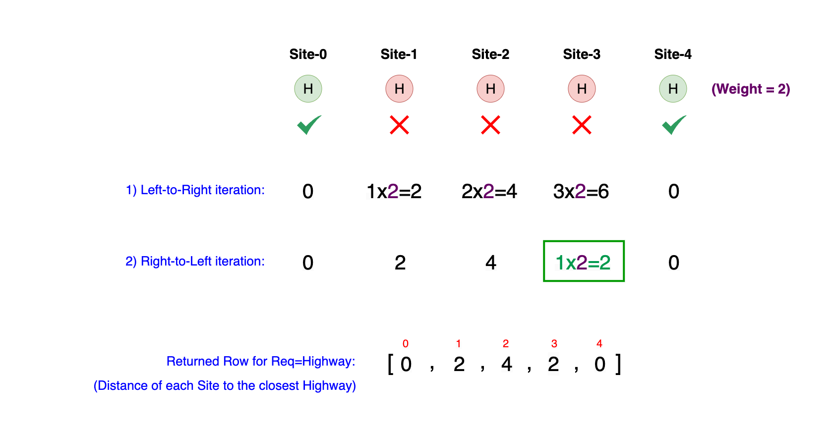
Let's consider our Example, and what the method calculate_min_distances(sites, "highway", 2) would return when the requirement is
"Highway" and its weight is 2. In the diagram below, sites with a "Highway" are marked in green, and those without are marked in red.
Performing a Left-to-Right iteration to update each site's closest distance to a "Highway", we observe that Site-0, which has a highway, sets its distance to 0. For Site-1, Site-2, and Site-3, the nearest "Highway" is at Site-0, resulting in distances of d=1*2=2, d=2*2=4, and d=3*2=6 respectively. As Site-4 also has its own "Highway", its distance is d=0.
Following the Left-to-Right scan, we next perform a Right-to-Left iteration. This step updates the minimum distances considering the proximity of requirements from the other direction. During this iteration, most sites retain their previously calculated distances, as Site-0 remains the closest site with a "Highway" for Site-1 and Site-2. However, there is a crucial update for Site-3. Initially, the nearest "Highway" was identified at Site-0 with a distance of d=3*2=6. But, looking from right to left, Site-3 is now closer to Site-4, which also has a "Highway". Hence, the distance for Site-3 is updated to d=1*2=2, significantly reducing its previously calculated distance. This adjustment highlights the importance of scanning from both directions to accurately assess the proximity of each site to the required services.
The image below demonstrates the returned row corresponding to the minimum distance of each site to requirement = "Highway".
This method, applied to each requirement, effectively pre-computes the minimum distance from every site to the closest site with the specified requirement, forming a critical part of our overall site evaluation strategy.
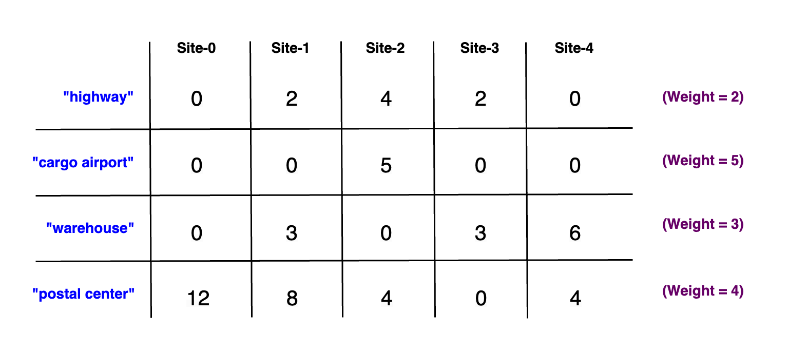
We repeat this process for each requirement, effectively constructing an (r x s) matrix, where r is the number of
requirements, and s is the total number of sites. This matrix serves as a comprehensive reference for our site evaluation.
In the matrix, each entry min_distances_from_sites[r][s] represents the minimum distance from site s to the requirement
r. The diagram below illustrates this pre-computed matrix, providing a clear overview of the distances from each site to
each requirement. Mind the weights applied to each distance!
2) Assessing Each Site's Overall Value to Decide the Optimal Site
The diagram above demonstrates our pre-computed min_distances_from_sites (r x s) array. It's crucial to understand what
this matrix represents and how it was constructed before moving to this section. Each cell in this array reflects the shortest
distance from a site (column) to a site that fulfills a specific requirement (row). This pre-computation is key to efficiently
assessing each site's overall value in terms of its proximity to all essential services.
This is where we consider the maximum of these pre-computed minimum distances for each site. The rationale is straightforward: the value of a site in this context is dictated by the farthest essential service. This "farthest service" becomes the bottleneck in terms of accessibility and hence is a critical factor in site selection.
The diagram below illustrates how we utilize the pre-computed min distances matrix. It's important to note that our focus now shifts to each column, as each column represents an individual site. Within a column, the maximum value is what dictates the value of that site. This maximum value represents the farthest essential service from the site, and finding the site with the smallest of these maximum values is our goal. This approach ensures we select a site that optimally balances proximity to all required services.
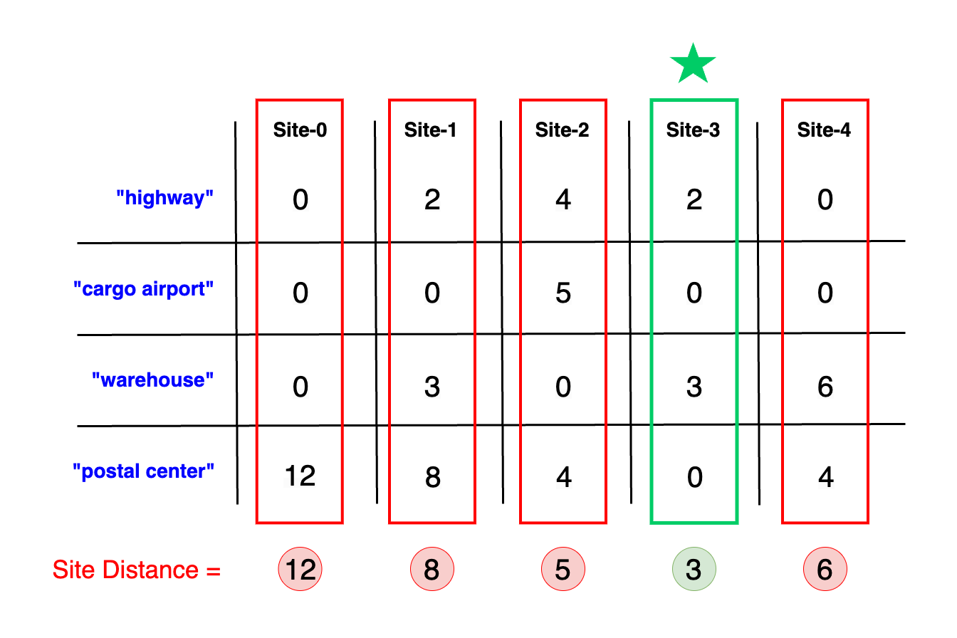
Observe that Site-3 has the smallest max distance to any of the requirements, equaling 3, making it the optimal site for Amazon Prime. This selection underscores the significance of the maximum distance and weights in our evaluation. Interestingly, while Site-0 possesses a highway, cargo airport, and a warehouse, almost positioning it as the best site, its distance to the nearest postal center is 12 (3 * 4). The max distance together with the requirement's weight ultimately render it the least favorable option among all sites.
Below is the code snippet that helps us utilize this pre-computed matrix to determine the maximum distance per site to any of the required services. This process is essential in identifying the optimal site:
Using Pre-Computed Matrix for further Computations
# After we find the min distance from each site to each requirement,
# we need to find the max distance per site.
# e.g., the overall max distances of each site to all requirements.
# e.g., max_distances_in_sites[s] ==> max(distanceBetween(s, req1), distanceBetween(s, req2)).
# Then, we need to select the minimum among those max values. Whichever site has the min value
# is the site we are looking for.
max_distances_in_sites = [0] * len(sites)
for s in range(len(sites)):
    for r in range(len(requirements)):
        # We already know the min distance of a particular site 's' to each and every 'req'.
        # We are interested in the max value because that's the value that Amazon is interested in.
        max_distances_in_sites[s] = max(max_distances_in_sites[s],
                                        min_distances_from_sites[r][s])

# Site with the min value is the optimal site.
return get_site_idx_with_min_val(max_distances_in_sites)
In this snippet, we iterate through each site and calculate the maximum distance to any requirement from that site, effectively finding the 'worst-case' scenario for each location. By selecting the site with the smallest maximum distance, we ensure the chosen site is optimally located with respect to all essential services, aligning with Amazon's operational efficiency goals.
In the diagram above, the max_distances_in_sites array is shown to be [12, 8, 5, 3, 6].
This array represents the maximum distance to any requirement for each site. The minimum max distance in
this array is 3, which belongs to
Site-3. This makes Site-3 the optimal choice for the Amazon Prime hub.
To identify this optimal site programmatically, we use the get_site_idx_with_min_val helper function.
This function iterates through the max_distances_in_sites = [12, 8, 5, 3, 6] array and efficiently determines the
index of the site with the smallest maximum distance, leading us to the best strategic location for the hub:
Finding the idx of the Site with the Smallest Distance
# O(n) time | O(1) space
# Helper function to return the idx of the site that has the smallest distance
# e.g., the answer we are looking for.
def get_site_idx_with_min_val(array):
    min_val_idx = 0
    min_val = float('inf')
    for i in range(len(array)):
        if array[i] < min_val:
            min_val = array[i]
            min_val_idx = i
    return min_val_idx
Complexity Analysis
-
Time Complexity: O(s × r), where s represents the number of sites, and r represents the number of different requirements to be checked for each site.
Explanation:
-
Pre-Computing Distances
- For each requirement r, we perform two linear scans (Left-to-Right and Right-to-Left) across all sites s.
- These scans are O(s) operations, and since we repeat them for each of the r requirements, the complexity for this part becomes O(s × r).
-
Evaluating Each Site
- After pre-computing the distances, we iterate over each site s.
- For each site, we iterate over all requirements r to find the maximum distance.
- This process is again an O(s × r) operation.
Combining both parts, the overall time complexity of the algorithm remains O(s × r), which represents a significant improvement over the more intuitive O(s² × r) solution.
-
-
Space Complexity: O(s × r). The space complexity is primarily determined by the storage requirements of the pre-computed distances, which are held in a 2D array (or matrix) with dimensions r (requirements) by s (sites).
Explanation:
-
Storing Minimum Distances
- The
min_distances_from_sitesmatrix is anr × smatrix, hence occupying O(s × r) space.
- The
-
Additional Arrays
- The
max_distances_in_sitesarray, although contributing to space complexity, is only of size s (one entry per site), which is comparatively smaller than the matrix and does not change the overall O(s × r) space complexity.
- The
-
In conclusion, while the space complexity increases to O(s * r) in this solution, this trade-off is justified by the considerable improvement in time efficiency, making the algorithm suitable for scenarios where quick processing is prioritized over memory usage.
Below is the coding solution for the advanced algorithm we've just discussed in Solution 2. This solution effectively demonstrates how we can leverage pre-computed minimum distances to evaluate each site's overall value to improve our time complexity to O(s * r).
# O(s * r) time | O(s * r) space
def optimal_site_search(sites, requirements, weights):
    # (r x s) array containing the minimum distance from each site to each requirement.
    # e.g., min_distances_from_sites[r][s] ==> minimum distance from site 's' to req 'r'.
    min_distances_from_sites = []
    for req_idx, req in enumerate(requirements):
        # Each iteration generates an array containing the min distance of each site to
        # the specific 'req' in the iteration.
        min_distances_from_sites.append(calculate_min_distances(sites, req, weights[req_idx]))

    # After we find the min distance from each site to each requirement,
    # we need to find the max distance per site.
    # e.g., the overall max distances of each site to all requirements.
    # e.g., max_distances_in_sites[s] ==> max(distanceBetween(s, req1), distanceBetween(s, req2)).
    # Then, we need to select the minimum among those max values. Whichever site has the min value
    # is the site we are looking for.
    max_distances_in_sites = [0] * len(sites)
    for s in range(len(sites)):
        for r in range(len(requirements)):
            # We already know the min distance of a particular site 's' to each and every 'req'.
            # We are interested in the max value because that's the value that Amazon is interested in.
            max_distances_in_sites[s] = max(max_distances_in_sites[s],
                                            min_distances_from_sites[r][s])

    # Site with the min value is the optimal site.
    return get_site_idx_with_min_val(max_distances_in_sites)

# O(s) time | O(s) space
# Helper function to calculate the min distance of each site to a particular req.
# We do a Left-to-Right and then Right-to-Left iterations to update the values in O(s) time.
def calculate_min_distances(sites, req, weight):
    min_distances_to_req = [float('inf')] * len(sites)
    site_with_min_dist_idx = float('inf')
    # Scan the min distances from Left to Right.
    for i in range(len(sites)):
        if sites[i][req] == 1:
            site_with_min_dist_idx = i
        min_distances_to_req[i] = abs(i - site_with_min_dist_idx) * weight

    # Update the min distances by scanning from Right to Left.
    for j in range(len(sites) - 1, -1, -1):
        if sites[j][req] == 1:
            site_with_min_dist_idx = j
        min_distances_to_req[j] = min(min_distances_to_req[j],
                                      abs(j - site_with_min_dist_idx) * weight)

    return min_distances_to_req

# O(n) time | O(1) space
# Helper function to return the idx of the site that has the smallest distance
# e.g., the answer we are looking for.
def get_site_idx_with_min_val(array):
    min_val_idx = 0
    min_val = float('inf')
    for i in range(len(array)):
        if array[i] < min_val:
            min_val = array[i]
            min_val_idx = i
    return min_val_idx
Final Notes
We believe the "Optimal Site for Amazon Prime Hub" question has appeared in recent Amazon software engineering interviews. It tests the candidate's ability to address complex logistical challenges through efficient algorithmic solutions.
As a prospective member of Amazon's dynamic logistics team, where decisions have substantial impacts on operational efficiency and customer satisfaction, mastering this problem provides valuable insights:
1) Strategic Logistic Planning: This challenge simulates the real-world task of identifying the most strategic location for a crucial distribution hub. It demonstrates the necessity of optimizing logistics planning for Amazon's vast and intricate supply chain network.
2) Balancing Time and Space Complexity: The transition from an intuitive O(s² × r) approach to a more sophisticated O(s × r) solution illustrates the importance of balancing time and space complexities. This is crucial in scenarios where timely data processing outweighs the cost of increased memory usage.
3) Algorithmic Efficiency and Practicality: Amazon values solutions that are not only theoretically sound but also practical and implementable. This problem underscores the need to develop algorithms that are efficient, scalable, and directly applicable to real-life challenges.
4) Understanding of Multidimensional Data Structures: The use of a 2D array to pre-compute distances reflects the need for proficiency in handling complex data structures. Such skills are essential for solving logistical problems that Amazon faces daily.
5) Problem-Solving and Critical Thinking: This question evaluates your problem-solving skills, particularly your ability to refine brute-force approaches into more efficient algorithms. It tests your critical thinking in optimizing key operational metrics.
6) Contextual Application of Solutions: Tailoring your algorithm to suit Amazon's operational needs showcases your ability to align technical solutions with business objectives. It reflects an understanding of how these solutions can directly impact Amazon's service quality and customer experience.
7) Clear Communication of Complex Ideas: Effectively articulating your solution strategy is crucial, especially in a diverse team environment like Amazon's. Your ability to clearly explain complex algorithms is indicative of your potential for collaborative problem-solving.
8) Focus on Customer-Centric Solutions: Amazon's leadership principles emphasize customer obsession. This problem, in its essence, is about enhancing customer experience through improved logistical efficiency, highlighting the importance of customer-centric decision-making in your solutions.
In preparing for a role at Amazon, especially within teams focused on logistics and operations, demonstrating your ability to develop and apply efficient algorithms to real-world challenges is key. This problem not only tests your technical skills but also your understanding of how these skills can be used to drive Amazon's operational excellence and customer satisfaction forward.
Embrace these challenges as opportunities to showcase your problem-solving capabilities and your alignment with Amazon's vision of constant innovation and customer focus. Good luck in your interview preparation, and may your solutions contribute to the next big leap in Amazon's operational strategies!